Developing LLM-integrated GIT vision language models.
Summary of this article:
Large language models (LLM) are showing their value more and more. Incorporating images into LLMs makes them even more useful as vision language models. In this article, I will explain the development of a model called GIT-LLM, a simple but powerful vision language model. Some parts, like the code explanations, might feel a bit tedious, so feel free to jump straight to the results section. I conducted various experiments and analyses, so I think you’ll enjoy seeing what I was able to achieve.
The implementation is available publicly, so please give it a try.
GitHub - turingmotors/heron
Transforming GIT into LLM
Let’s dive into the main topic of this tech blog.
What is GIT?
Generative Image-to-text Transformer, or GIT, is a vision language model proposed by Microsoft.
arXiv: https://arxiv.org/abs/2205.14100
Code: https://github.com/microsoft/GenerativeImage2Text
Its architecture is quite simple. It converts feature vectors extracted from an image encoder into vectors that can be treated like text using a projection module. These vectors are then input into a language model to produce captions for images or to perform Q&A. The model can handle videos in a similar way.
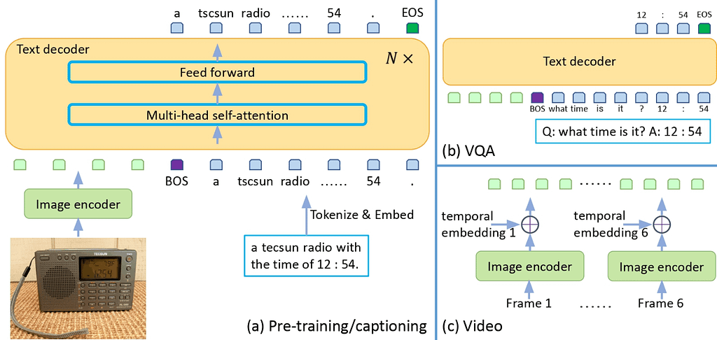
This figure is cited from “GIT: A Generative Image-to-text Transformer for Vision and Language”
Despite its simplicity, if you look at the Leaderboard on “Paper with code”, you’ll find that it ranks highly in many tasks.
https://paperswithcode.com/paper/git-a-generative-image-to-text-transformer
Originally, GIT uses strong models like CLIP for its image encoder and trains the language model part from scratch. However, in this article, I try to use a powerful LLM and fine-tune it. Here, I call the model “GIT-LLM”.
Using a LLM with Hugging Face’s Transformers
I’ll use Hugging Face’s Transformers library for developping GIT-LLM. Transformers is a Python library for handling machine learning models. It offers many state-of-the-art pre-trained models that you can immediately run inference on. It also provides tools for training and fine-tuning models. I believe that Transformers has contributed significantly to the development of recent LLM derivatives. Almost all available LLMs can be handled with Transformers, and many multi-modal models derived from them use Transformers as their base for development and fine-tuning.
Here is the simplest code for using a model of Transformers. You can find it easy to try LLMs by useing AutoModel and AutoTokenizer.
from transformers import AutoModelForCausalLM, AutoTokenizer
model_name = "facebook/opt-350m"
model = AutoModelForCausalLM.from_pretrained(model_name).to("cuda")
tokenizer = AutoTokenizer.from_pretrained(model_name)
prompt = "Hello, I'm am conscious and"
input_ids = tokenizer(prompt, return_tensors="pt").to("cuda")
sample = model.generate(**input_ids, max_length=64)
print(tokenizer.decode(sample[0]))
# Hello, I'm am conscious and I'm a bit of a noob. I'm looking for a good place to start.
Let’s check out the parameters the OPT model holds. Printing a model created by AutoModelForCausalLM.
OPTForCausalLM(
(model): OPTModel(
(decoder): OPTDecoder(
(embed_tokens): Embedding(50272, 512, padding_idx=1)
(embed_positions): OPTLearnedPositionalEmbedding(2050, 1024)
(project_out): Linear(in_features=1024, out_features=512, bias=False)
(project_in): Linear(in_features=512, out_features=1024, bias=False)
(layers): ModuleList(
(0-23): 24 x OPTDecoderLayer(
(self_attn): OPTAttention(
(k_proj): Linear(in_features=1024, out_features=1024, bias=True)
(v_proj): Linear(in_features=1024, out_features=1024, bias=True)
(q_proj): Linear(in_features=1024, out_features=1024, bias=True)
(out_proj): Linear(in_features=1024, out_features=1024, bias=True)
)
(activation_fn): ReLU()
(self_attn_layer_norm): LayerNorm((1024,), eps=1e-05, elementwise_affine=True)
(fc1): Linear(in_features=1024, out_features=4096, bias=True)
(fc2): Linear(in_features=4096, out_features=1024, bias=True)
(final_layer_norm): LayerNorm((1024,), eps=1e-05, elementwise_affine=True)
)
)
)
)
(lm_head): Linear(in_features=512, out_features=50272, bias=False)
)
It’s quite simple. The input dimension of the initial embed_tokens and the output dimension of the final lm_head is 50,272, which represents the number of tokens used in training this model. Let’s verify the size of the tokenizer’s vocabulary:
print(tokenizer.vocab_size)
# 50265
Including special tokens like bos_token, eos_token, unk_token, sep_token, pad_token, cls_token, and mask_token, it predicts the probability of the next word from a total of 50,272 types of tokens.
You can understand how these models are connected by looking at the implementation. A simple diagram would represent the flow as follows:
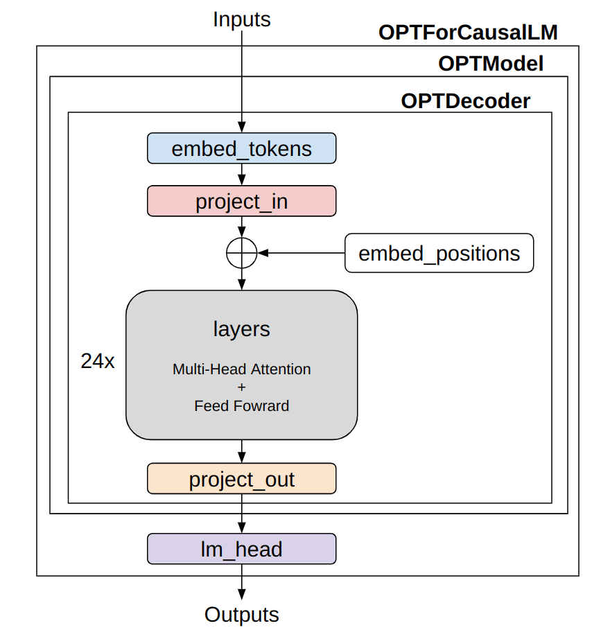
Simplified model architecture of OPT (image made by the author)
The structure and data flow are quite simple. The 〇〇Model and 〇〇ForCausalLM have a similar framework across different language models. The 〇〇Model class mainly represents the “Transformer” part of the language model. If, for instance, you want to perform tasks like text classification, you’d use only this part. The 〇〇ForCausalLM class is for text generation, applying a classifier for token count to the vectors after processing them with the Transformer. The calculation of the loss is also done within the forward method of this class. The embed_positions denotes positional encoding, which is added to project_in.
Using GIT with Transformers
I’ll give it a try based on the official documentation page of GIT. As I’ll be processing images as well, I’ll use a Processor that also includes a Tokenizer.
from PIL import Image
import requests
from transformers import AutoProcessor, AutoModelForCausalLM
model_name = "microsoft/git-base-coco"
model = AutoModelForCausalLM.from_pretrained(model_name)
processor = AutoProcessor.from_pretrained(model_name)
# Downloading and preprocess an image
url = "http://images.cocodataset.org/val2017/000000039769.jpg"
image = Image.open(requests.get(url, stream=True).raw)
pixel_values = processor(images=image, return_tensors="pt").pixel_values
# Preprocessing text
prompt = "What is this?"
inputs = processor(
prompt,
image,
return_tensors="pt",
max_length=64
)
sample = model.generate(**inputs, max_length=64)
print(processor.tokenizer.decode(sample[0]))
# two cats sleeping on a couch
Given that the input image produces the output “two cats sleeping on a couch”, it seems to be working well.
Let’s also take a look at the model’s structure:
GitForCausalLM(
(git): GitModel(
(embeddings): GitEmbeddings(
(word_embeddings): Embedding(30522, 768, padding_idx=0)
(position_embeddings): Embedding(1024, 768)
(LayerNorm): LayerNorm((768,), eps=1e-12, elementwise_affine=True)
(dropout): Dropout(p=0.1, inplace=False)
)
(image_encoder): GitVisionModel(
(vision_model): GitVisionTransformer(
...
)
)
(encoder): GitEncoder(
(layer): ModuleList(
(0-5): 6 x GitLayer(
...
)
)
)
(visual_projection): GitProjection(
(visual_projection): Sequential(
(0): Linear(in_features=768, out_features=768, bias=True)
(1): LayerNorm((768,), eps=1e-05, elementwise_affine=True)
)
)
)
(output): Linear(in_features=768, out_features=30522, bias=True)
)
Although it’s a bit lengthy, if you break it down, it’s also quite simple. Within GitForCausalLM, there is a GitModel and within that, there are the following modules:
The major difference from OPT is the presence of GitVisionModel and GitProjection, which are the exact modules that convert images into prompt-like vectors. While the language model uses a Decoder for OPT and an Encoder for GIT, this only signifies a difference in how the attention mask is constructed. There may be slight differences in the transformer layer, but their functions are essentially the same. GIT uses the name Encoder because it uses a unique attention mask that applies attention to all features of the image and uses a causal mask for text features.
Looking at the model’s connections;
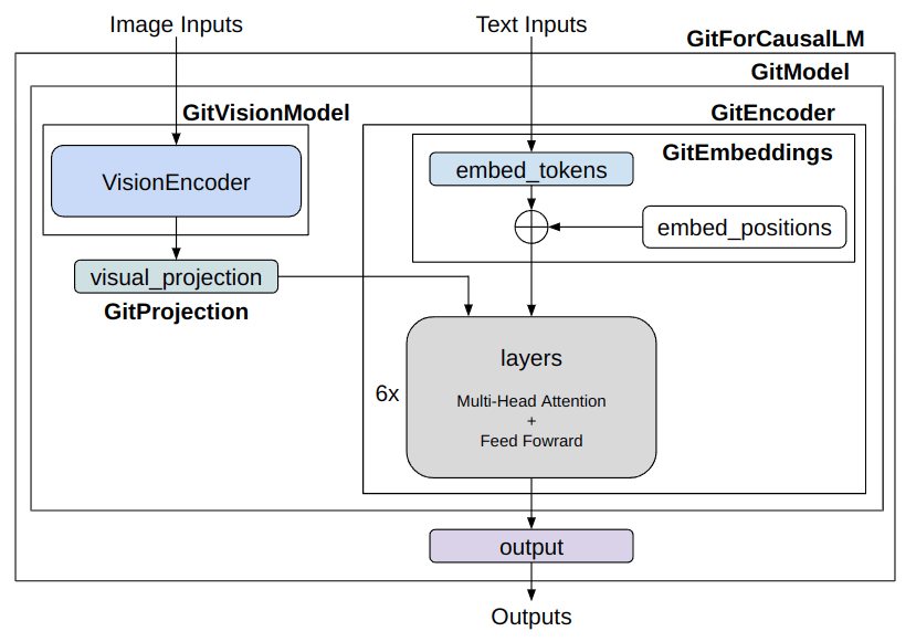
Simplified model architecture of GIT ( image made by the author)
The image information is treated by the GitVisionModel and GitProjection to match the text’s embeddings. After that, it’s inputted alongside the text’s embeddings into the language model’s “Transformer” layers. While there are subtle differences, the part related to the language model is almost developed the same way.
GIT’s Attention Mask
The architectures for the usual language model and the GIT language model are almost the same, but the ways of applying attention masks aredifferent.
For the language model, an attention mask is applied not to look at past tokens when predicting future tokens. This is a method called “Causal Attention”, which corresponds to the left side of the following figure. The first column token references only itself, ensuring no self attention is applied to subsequent words. The second column applies self attention up to the second word, with the third word onwards becoming 0. Such masking enables it to be trained to predict the next word effectively.
GIT input has two types of tokens: image tokens and text tokens. Since all image tokens are used simultaneously and aren’t used to predict the next token, Causal Attention isn’t suitable. On the other hand, Causal Attention is still necesarry for text tokens. A mask like the one on the right side of the figure is designed to achieve this. For the top three rows of image information, self attention is applied with all token information. From the text tokens, moving down one column increases the number of words that can be referenced.
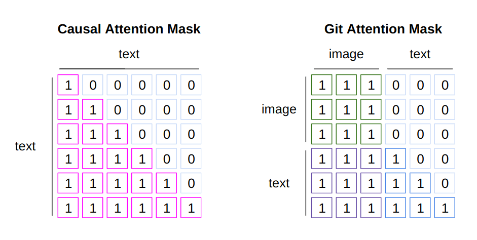
Difference between the causal attention mask and the Git attention mask (image made by the author)
Let’s also check the code for making a GIT mask. The snippet to create the GIT mask is as follows:
import torch
def create_git_attention_mask(
tgt: torch.Tensor,
memory: torch.Tensor,
) -> torch.Tensor:
num_tgt = tgt.shape[1]
num_memory = memory.shape[1]
# Areas where attention is applied are 0, areas without attention are -inf
top_left = torch.zeros((num_memory, num_memory))
top_right = torch.full(
(num_memory, num_tgt),
float("-inf"),
)
bottom_left = torch.zeros(
(num_tgt, num_memory),
)
# Causal Attention Mask
bottom_right = torch.triu(torch.ones(tgt.shape[1], tgt.shape[1]), diagonal=1)
bottom_right = bottom_right.masked_fill(bottom_right == 1, float("-inf"))
# Concatenate masks
left = torch.cat((top_left, bottom_left), dim=0)
right = torch.cat((top_right, bottom_right), dim=0)
# add axis for multi-head
full_attention_mask = torch.cat((left, right), dim=1)[None, None, :]
return full_attention_mask
# batch_size, sequence, feature_dim
visual_feature = torch.rand(1, 3, 128)
text_feature = torch.rand(1, 4, 128)
mask = create_git_attention_mask(tgt=text_feature, memory=visual_feature)
print(mask)
"""
tensor([[[[0., 0., 0., -inf, -inf, -inf, -inf],
[0., 0., 0., -inf, -inf, -inf, -inf],
[0., 0., 0., -inf, -inf, -inf, -inf],
[0., 0., 0., 0., -inf, -inf, -inf],
[0., 0., 0., 0., 0., -inf, -inf],
[0., 0., 0., 0., 0., 0., -inf],
[0., 0., 0., 0., 0., 0., 0.]]]])
"""
You add the mask to attention weights. Thus, parts where self attention takes place are 0, and parts that aren’t included in the attention are -inf. By providing this mask forward, only the text part can do causal attention. It’s important for vision language models to create and use masks effectively like this.
Connecting GIT and OPT
Now, let’s connect GIT and OPT. The goal is to create a model as shown in the figure.
Simplified model architecture of GIT-OPT (image made by the author)
For the general implementation, you can refer to the modeling_git.py.
The most important part is the GitOPTModel. Inside this, a vision encoder need to be connected with a LLM. I’ll explain some key components.
class GitOPTModel(OPTModel):
def __init__(self, config: OPTConfig):
super(GitOPTModel, self).__init__(config)
self.image_encoder = CLIPVisionModel.from_pretrained(config.vision_model_name)
self.visual_projection = GitProjection(config)
Inside the __init__ function, various modules are instantiated. The super initializes the OPTModel. In GIT, it is recommended to use a powerful image encoder trained with CLIP, so I have made it compatible with the ViT trained with CLIP. The GitProjection is taken from the original GIT implementation.
Let’s look inside the forward function. The implementation is based on the forward part of the OPTDecoder, with added information from the image encoder. Although it’s a bit lengthy, I’ve added comments in the code, so please follow each step.
class GitOPTModel(OPTModel):
...
def forward(
self,
input_ids: Optional[torch.Tensor] = None,
attention_mask: Optional[torch.Tensor] = None,
pixel_values: Optional[torch.Tensor] = None,
) -> BaseModelOutputWithPooling:
seq_length = input_shape[1]
# 1. Extract image features using ViT
visual_features = self.image_encoder(pixel_values).last_hidden_state
# 2. Convert features extracted by ViT into prompt-like Image Embeddings
projected_visual_features = self.visual_projection(visual_features)
# 3. Vectorize the tokens
inputs_embeds = self.decoder.embed_tokens(input_ids)
# 4. Obtain Positional Encoding
pos_embeds = self.embed_positions(attention_mask, 0)
# 5. Dimension adjustment of Text Embeddings specific to OPT
inputs_embeds = self.decoder.project_in(inputs_embeds)
# 6. Text Embeddings + Positional Encoding
embedding_output = inputs_embeds + pos_embeds
# 7. Concatenate Image Embeddings and Text Embeddings
hidden_states = torch.cat((projected_visual_features, embedding_output), dim=1)
# 8. Create Causal Attention Mask for Text region
tgt_mask = self._generate_future_mask(
seq_length, embedding_output.dtype, embedding_output.device
)
# 9. Create Attention Mask for GIT
combined_attention_mask = self.create_attention_mask(
tgt=embedding_output,
memory=projected_visual_features,
tgt_mask=tgt_mask,
past_key_values_length=0,
)
# 10. Pass through the Decoder layer repeatedly, the main part of the language model
for idx, decoder_layer in enumerate(self.decoder.layers):
layer_outputs = decoder_layer(
hidden_states,
attention_mask=combined_attention_mask,
output_attentions=output_attentions,
use_cache=use_cache,
)
hidden_states = layer_outputs[0]
# 11. Dimension adjustment MLP specific to OPT
hidden_states = self.decoder.project_out(hidden_states)
# 12. Align the output interface
return BaseModelOutputWithPast(
last_hidden_state=hidden_states,
past_key_values=next_cache,
hidden_states=all_hidden_states,
attentions=all_self_attns,
)
Although it might look complicated, if you go through each step, you’ll see that it follows the flow illustrated in the diagram. The actual code may look a bit more complex, but grasping the main process first will make understanding the other parts easier. This is pseudocode, so for detailed parts, please refer to the published implementation.
Finally, let’s take a brief look at the GITOPTForCausalLM part.
class GitOPTForCausalLM(OPTForCausalLM):
def __init__(
self,
config,
):
super(GitOPTForCausalLM, self).__init__(config)
self.model = GitOPTModel(config)
def forward(
...
) -> CausalLMOutputWithPast:
outputs = self.model(
...
)
sequence_output = outputs[0]
logits = self.lm_head(sequence_output)
loss = None
if labels is not None:
# Predict the next word as the task
num_image_tokens = self.image_patch_tokens
shifted_logits = logits[:, num_image_tokens:-1, :].contiguous()
labels = labels[:, 1:].contiguous()
loss_fct = CrossEntropyLoss()
loss = loss_fct(shifted_logits.view(-1, self.config.vocab_size), labels.view(-1))
return CausalLMOutputWithPast(
loss=loss,
logits=logits,
...
)
The processing inside the model is simple. When labels are provided, i.e., during training, the loss calculation is also performed within the forward. In shifted_logits, tokens were fetched from the first token to the second-to-last token of the text tokens. It then calculates the Cross Entropy Loss with the labels shifted by one word as the correct answer.
One thing to note is to name the variable that assigns the GitOPTModel in the initialization function as self.model. If you check the implementation of the parent class OPTForCausalLM, you'll see that OPT is first placed to self.model during the super initialization. If you change this instance variable name, you will end up holding two OPTs, which can strain the memory.
LoRA Extension
In order to fine-tune the LLM effectively, I’ll use a library called Parameter-Efficient Fine-Tuning (PEFT). As it’s developed by Hugging Face, it integrates seamlessly with Transfors. While there are various methods within PEFT, this time I’m going to do some experiments using a commonly seen approach called Low-rank adaptation (LoRA).
Models can be applied LoRA in just a few lines if the models support PEFT.
from transformers import AutoModelForCausalLM
from peft import get_peft_config, get_peft_model, LoraConfig
model = AutoModelForCausalLM.from_pretrained('microsoft/git-base')
peft_config = LoraConfig(
task_type="CAUSAL_LM",
r=8,
lora_alpha=32,
lora_dropout=0.1,
target_modules=["v_proj"]
)
peft_model = get_peft_model(model, peft_config)
The target_modules argument specifies which modules you want to convert to LoRA. If a list is provided as target_modules, it is implemented to convert to LoRA for modules that end with each of the strings. LoRA is applied only to “value” (v_proj) of the self attention module for simplicity.
In the model, ViT is used for the image encoder part. Be cautious, as specifying it like this, self attention part of ViT might also be applied LoRA. It’s a bit tedious, but by specifying down to the part where the key names don’t overlap and giving it to target_modules, you can avoid this.
target_modules = [f"model.image_encoder.vision_model.encoder.{i}.self_attn.v_proj" for i in range(len(model.model.decoder))]
The resulting model becomes an instance of the PeftModelForCausalLM class. It has an instance variable named base_model that holds the original model converted to LoRA. As an example, I show that LoRA is applied to v_proj of the self attention in ViT.
(self_attn): GitVisionAttention(
(k_proj): Linear(in_features=768, out_features=768, bias=True)
(v_proj): Linear(
in_features=768, out_features=768, bias=True
(lora_dropout): ModuleDict(
(default): Dropout(p=0.1, inplace=False)
)
(lora_A): ModuleDict(
(default): Linear(in_features=768, out_features=8, bias=False)
)
(lora_B): ModuleDict(
(default): Linear(in_features=8, out_features=768, bias=False)
)
(lora_embedding_A): ParameterDict()
(lora_embedding_B): ParameterDict()
)
(q_proj): Linear(in_features=768, out_features=768, bias=True)
(out_proj): Linear(in_features=768, out_features=768, bias=True)
)
Inside the v_proj Linear, you'll find added fully connected layers such as lora_A and lora_B. The LoRA-converted Linear module is a namesake Linear class that inherits from PyTorch's Linear and LoraLayer. It's a somewhat unique module, so those curious about the details should take a look at the implementation.
Note that models created with PEFT will not save anything other than the LoRA part by default. While there’s a method to save using the merge_and_unload method, you might want to save all models being saved midway during training with Trainer. Overloading the Trainer's _save_checkpoints method is one approach, but to avoid the hassle, I handled it this time by fetching just the original model part held inside the PeftModel during the training phase.
model = get_peft_model(model, peft_config)
model.base_model.model.lm_head = model.lm_head
model = model.base_model.model
I believe there are more efficient ways to handle this, so I’m still researching.
Experimenting with GIT-LLM
Let’s now conduct some experiments using the model developed so far.
For details on the training configuration and other setups, please refer to the published implementation, as they essentially follow the same method.
Dataset: M3IT
For experiments, I wanted to use a dataset that pairs images with text and is easy to integrate. While exploring the Hugging face’s Datasets, I came across M3IT, a multimodal dataset for Instruction Tuning developed by the Shanghai AI Lab. Instruction Tuning is a method that yields impressive results even with a limited amount of data. It appears that M3IT has re-annotated various existing datasets specifically for Instruction Tuning.
https://huggingface.co/datasets/MMInstruction/M3IT
This dataset is easy to use, so I’ve decided to utilize it for the following experiments.
To train using M3IT, it’s necessary to create a custom Pytorch Dataset.
class SupervisedDataset(Dataset):
def __init__(
self,
vision_model_name: str,
model_name: str,
loaded_dataset: datasets.GeneratorBasedBuilder,
max_length: int = 128,
):
super(SupervisedDataset, self).__init__()
self.loaded_dataset = loaded_dataset
self.max_length = max_length
self.processor = AutoProcessor.from_pretrained("microsoft/git-base")
# Setting up the corresponding Processor for each model
self.processor.image_processor = CLIPImageProcessor.from_pretrained(vision_model_name)
self.processor.tokenizer = AutoTokenizer.from_pretrained(
model_name, padding_side="right", use_fast=False
)
def __len__(self) -> int:
return len(self.loaded_dataset)
def __getitem__(self, index) -> dict:
# cf: https://huggingface.co/datasets/MMInstruction/M3IT#data-instances
row = self.loaded_dataset[index]
# Creating text input
text = f'##Instruction: {row["instruction"]} ##Question: {row["inputs"]} ##Answer: {row["outputs"]}'
# Loading the image
image_base64_str_list = row["image_base64_str"] # str (base64)
img = Image.open(BytesIO(b64decode(image_base64_str_list[0])))
inputs = self.processor(
text,
img,
return_tensors="pt",
max_length=self.max_length,
padding="max_length",
truncation=True,
)
# batch size 1 -> unbatch
inputs = {k: v[0] for k, v in inputs.items()}
inputs["labels"] = inputs["input_ids"]
return inputs
In the __init__ function, the image_processor and tokenizer correspond to their respective models. The loaded_dataset argument passed should be from MMInstruction/M3IT datasets.
coco_datasets = datasets.load_dataset("MMInstruction/M3IT", "coco")
test_dataset = coco_datasets["test"]
For the COCO Instruction Tuning dataset, the split between training, validation, and testing is identical to the original dataset, with 566,747, 25,010, and 25,010 image-text pairs respectively. Other datasets, such as VQA or Video, can also be handled similarly, making it a versatile dataset for validation purposes.
A sample data looks like this:

Image is cited from data in M3IT.
The caption for this picture is as follows:
For the COCO dataset, which is for Captions, the Question portion is left blank.
Let’s delve deeper into the processor’s operations. Essentially, it normalizes images and tokenizes text. Inputs shorter than max_length are also padded. The processed data returned by the processor is a dictionary containing:
These key names correspond to the arguments for the model’s forward function, so they shouldn’t be altered. Finally, input_ids are directly passed to a key named labels. The forward function of GitOPTForCausalLM calculates the loss by predicting the next word shifted by one token.
Experiment 1: Determining Fine-tuning Locations
In the research papers on GIT models, it was explained that a strong vision encoder is utilized and random parameters are adopted for the language model. This time, since the goal is to ultimately use a 7B-class language model, a pre-trained model will be applied to the language model. The following modules will be examined for fine-tuning. The GIT Projection, being an initialized module, is always included. Some combinations may seem redundant, but they are explored without too much concern for this trial.
Modules set for training are given gradients, while the rest are modified to not have gradients.
# Specifying the parameters to train (training all would increase memory usage)
for name, p in model.model.named_parameters():
if np.any([k in name for k in keys_finetune]):
p.requires_grad = True
else:
p.requires_grad = False
The Vision Encoder and LLM used for this examination are:
Training utilizes COCO dataset and lasts for 5 epochs.
Here are the target modules trained during each experiment:
(Note: While LoRA can be applied to ViT, but to avoid making the experiments too complicated, it wasn’t included this time.)
This figure shows training loss. Proj, LoRA, OPT, ViT, and Head in the legend are the trained modules explained above. (figure made by the author)
As shown in the training loss plot, it’s apparent that some groups are not performing well. These were the case when OPT is included in the training. Although all experiments were conducted under fairly similar conditions, more detailed adjustments, such as learning rate, might be necessary when fine-tuning the language model. Results, excluding the models where OPT is included in training, will be examined next.

This figure shows training loss without full finetuning results. Proj, LoRA, OPT, ViT, and Head in the legend are the trained modules explained above. (figure made by the author)
This figure shows validation loss. Proj, LoRA, OPT, ViT, and Head in the legend are the trained modules explained above. (figure made by the author)
Both training and validation Loss decreased most with the Projection+LoRA model. Fine-tuning final Head layer showed nearly identical outcomes. If ViT is also trained, the Loss appears slightly higher and results seem unstable. Even when adding LoRA during ViT training, the loss still tends to be high. For fine-tuning with this data, it seems using a pre-trained ViT model without updating its parameters yields more stable results. The effectiveness of LoRA has been acknowledged in various places, and it is evident from this experiment that adding LoRA to the LLM improved bothe traininng and validation loss.
Reviewing the inference results on some test data:
Example results of GIT-OPT. Pictures are cited from M3IT dataset, and text results were made by the author’s model
When training OPT itself, the results are as poor as the result of loss, making the model at a loss for words. Additionally, when training ViT, the output makes semantic sense, but describes something entirely different from the given image. However, the other results seem to capture the features of the images to some extent. For instance, the first image mentions “cat” and “banana”, and the second one identifies “traffic sign”. Comparing results with and without LoRA, the latter tends to repetitively use similar words, but using LoRA seems to make it slightly more natural. Training the Head results in intriguing outputs, like using “playing” instead of “eating” for the first image. While there are some unnatural elements in these results, it can be deduced that the training was successful in capturing image features.
Experiment 2: Comparing Billion-Scale Models
For fine-tuning conditions in earlier experiments, a slightly smaller language model, OPT-350m, was used. Now, the intention is to switch the language model to a 7B model. Not just settling for OPT, stronger LLMs, LLaMA and MPT, will also be introduced.
Integrating these two models can be done in a similar fashion to OPT. Referring to the forward functions of the LlamaModel and MPTModel, combine the projected image vectors with text tokens, and change the mask from Causal Attention Mask to GIT’s Attention Mask. One thing to note: for MPT, the mask isn’t (0, -inf), but (False, True). The subsequent processes can be implemented similarly.
To use the 7B-class model with OPT, merely change the model name from facebook/opt-350m to facebook/opt-6.7b.
For LLaMA, with the availability of LLaMA2, that will be the model of choice. To use this pre-trained model, approvals from both Meta and Hugging Face are needed. An account is necessary for Hugging Face, so make sure to set that up. Approvals typically come within a few hours. Afterwards, log into Hugging Face on the terminal where training is executed.
huggingface-cli login
You can log in using the token created in Hugging Face account → Settings → Access Token.
Training parameters remain consistent, using the COCO dataset and lasting for 3 epochs. Based on results from Experiment 1, the modules set for fine-tuning were Projection + LoRA.
Let’s take a look at the results.
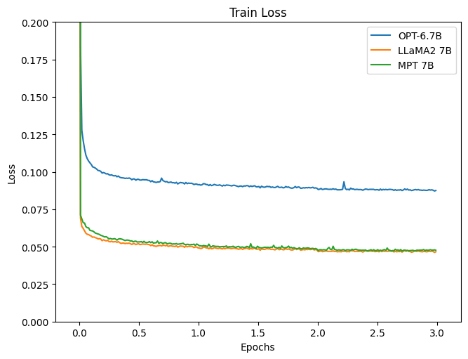
This figure shows training loss (figure made by the author)
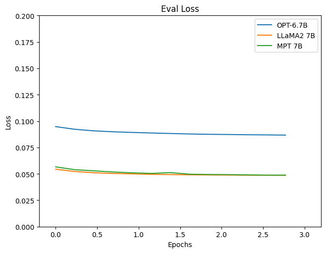
This figure shows validation loss (figure made by the author)
Reviewing the loss, it’s apparent that the models using LLaMA2 and MPT as LLM show a more satisfactory reduction. Let’s also observe the inference results.
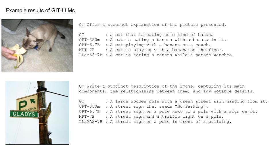
Example results of GIT-LLMs. Pictures are cited from M3IT dataset, and text results were made by the author’s model
Regarding the first image, for all models, the expressions seem more natural compared to OPT-350m. There are no bizarre expressions like “a banana with a banana”, highlighting the strength of LLM. For the second image, there’s still some difficulty with phrases like “a traffic light” or “a building”. For such complex images, there might be a need to consider upgrading the ViT model.
Finally, let’s run inference on images that became popular with GPT-4.

Example results of GIT-LLMs. A picture is cited from here, and text results were made by the author’s models
Although fluent responses were anticipated since LLM is in use, the outcomes are quite simple. This might be because the model was trained solely on COCO.
Experiment 3. Increasing the Data
Given the underwhelming results of the previous experiment, it was decided to incorporate data other than COCO for training. The M3IT dataset currently in use is quite comprehensive, and it can handle a significant amount of data in the same format as COCO.
This table is cited from Table 3 of “M3IT: A Large-Scale Dataset towards Multi-Modal Multilingual Instruction Tuning”
It is intended to use data from this source excluding the “Chinese” and “Video” categories. Originally, the COCO training dataset contained 566,747 pieces of data. By combining it with additional sources, this increased to 1,361,650. Although the size has roughly doubled, the dataset is believed to have become of higher quality due to the increased diversity of tasks.
Handling multiple Pytorch datasets can be easily achieved using the ConcatDataset.
dataset_list = [
datasets.load_dataset("MMInstruction/M3IT", i) for i in m3it_name_list
]
train_dataset = torch.utils.data.ConcatDataset([d["train"] for d in dataset_list])
The training was conducted for 1 epoch, and the LLaMA2 model was used for fine-tuning the Projection and LoRA, similarly to Experiment 2.
As there’s no loss to compare to this time, let’s dive straight into the inference results.

Example results of GIT-LLaMA2. Pictures are cited from M3IT dataset, and text results were made by the author’s model
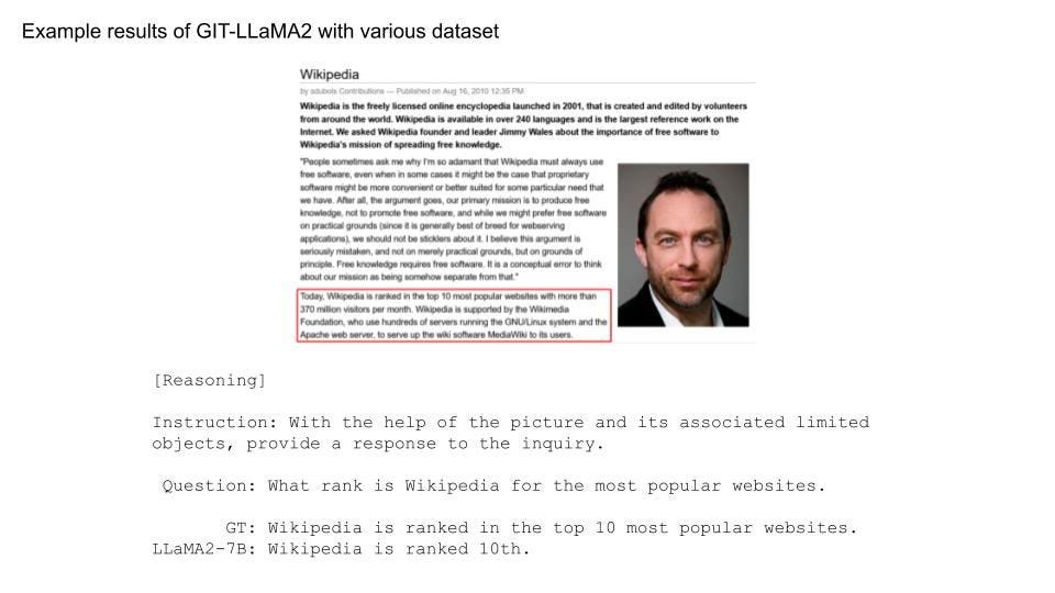
Example results of GIT-LLaMA2. Pictures are cited from M3IT dataset, and text results were made by the author’s model
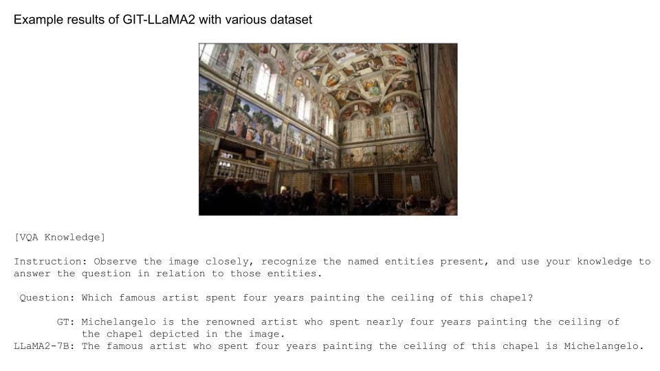
Example results of GIT-LLaMA2. Pictures are cited from M3IT dataset, and text results were made by the author’s model
Along with solving simple problems, the model now handles more complex challenges. By adding datasets for tasks more intricate than just captioning, the capabilities have expanded significantly. Achieving this level of accuracy with only 1 epoch of training was surprising.
Let’s test it with the following example image. Given the increased variety in the dataset, the way the questions were presented was slightly modified.
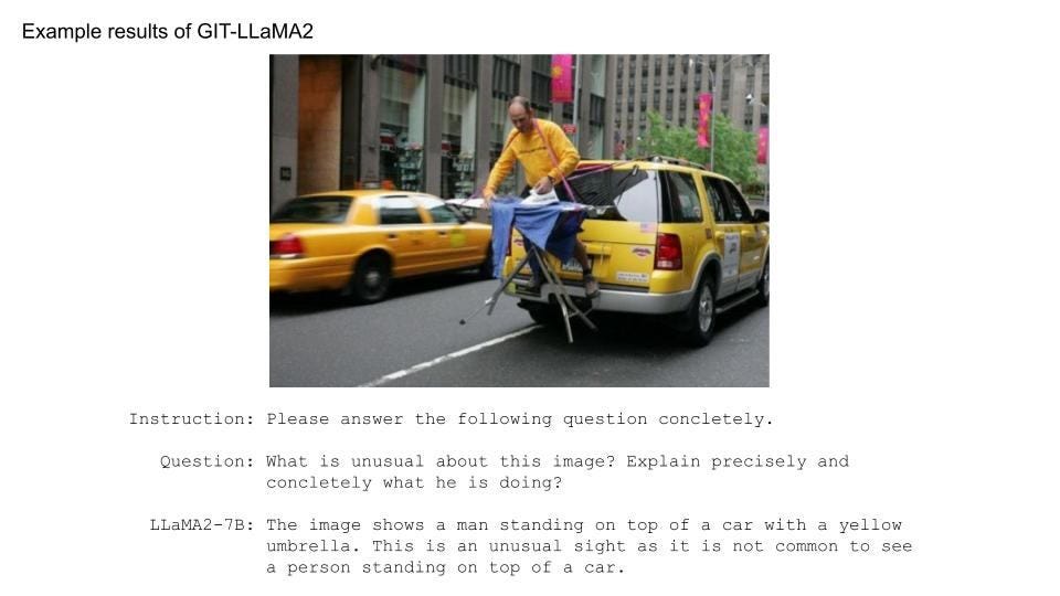
Example results of GIT-LLaMA2. A picture is cited from here, and text results were made by the author’s models
While the description being “Umbrella” was still wired, it feels like it’s getting better. To improve further, there’s a need to increase the number of training epochs, add more types or volumes of datasets, and leverage more powerful ViT or LLM. Nonetheless, it’s impressive that such a model could be developed in just half a day given the computational and data resources.
Bonus Experiment. Did the Image Turn into Words?
Let’s take another look at the GIT structure.
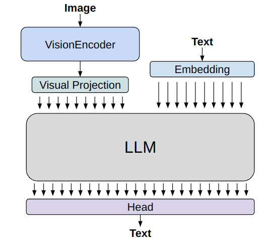
Simplified model architecture of GIT-LLM (image made by the author)
As shown in the figure, after feature extraction by the vision encoder, images are treated on par with vectorized text through Visual Projection. In other words, it’s possible that the Visual Projection is converting image vectors into text vectors. An investigation was conducted to see what the vectors look like after theVisual Projection.
While there’s an option to use the Head to revert the vector post-projection back to text, it was found that even vectors that were vectorized using the Embedding module could not be reverted back to their original text using this method. Therefore, vectors that closely resemble the text vectors before being input into the LLM should be assigned as the corresponding word. All tokens registered in the tokenizer were vectorized using the Embedding module, and the one with the highest cosine similarity was identified as the target word.
The image used for this experiment is that of a cat.
A Picture is cited from M3IT dataset.
Now, let’s proceed with the analysis (whole analysis is available here). First, all the registered tokens are vectorized.
coco_datasets = datasets.load_dataset("MMInstruction/M3IT", "coco")
test_dataset = coco_datasets["test"]
supervised_test_dataset = SupervisedDataset(model_name, vision_model_name, test_dataset, 256)
ids = range(supervised_test_dataset.processor.tokenizer.vocab_size)
all_ids = torch.tensor([i for i in ids]).cuda()
token_id_to_features = model.model.embed_tokens(all_ids)
Next, the image vectors that would have been converted to words by the ViT and Projection are extracted.
inputs = supervised_test_dataset[0] # Picking a sample arbitrarily
pixel_values = inputs["pixel_values"]
out_vit = model.model.image_encoder(pixel_values).last_hidden_state
out_vit = model.model.visual_projection(out_vit)
The dot products of these vectors and the word vectors were calculated, and the results with the maximum value were decoded as the relevant token ID.
# Dot product
nearest_token = out_vit[0] @ token_id_to_features.T
# The index of the maximum value corresponds to the relevant token ID
visual_out = nearest_token.argmax(-1).cpu().numpy()
decoded_text = supervised_test_dataset.processor.tokenizer.batch_decode(visual_out)
print(decoded_text)
"""
['otr', 'eg', 'anto', 'rix', 'Nas', ...]
"""
As shown in the printed decoded_text, some unfamiliar words have appeared. As some words are repeated, they were counted.
print(pd.Series(decoded_text).value_counts())
"""
mess 43
atura 29
せ 10
Branch 10
Enum 9
bell 9
worden 7
...
"""
A large number of unfamiliar words seem to have appeared. Depending on the position, they might convey meaningful information. Let’s plot the words against the cat image.
n_patches = 14
IMAGE_HEIGHT = 468
IMAGE_WIDTH = 640
y_list = np.arange(15, IMAGE_HEIGHT, IMAGE_HEIGHT//n_patches)
x_list = np.arange(10, IMAGE_WIDTH, IMAGE_WIDTH//n_patches)
plt.figure()
plt.axis("off")
plt.imshow(np.array(image), alpha=0.4)
for index in np.arange(n_patches ** 2):
y_pos = index // n_patches
x_pos = index - y_pos * n_patches
y = y_list[y_pos]
x = x_list[x_pos]
# The first token is the bos token, so it is excluded
word = decoded_text[index + 1]
# For differentiating words by color
plt.annotate(word, (x, y), size=7, color="blue")
plt.show()
plt.clf()
plt.close()

Image made by the author
Words that frequently appear are color-coded. The result seems to suggest that they are not simply being projected onto meaningful words. While the word “Cat” might be superimposed on the cat image, giving it some relevance, its meaning remains unclear.
The inconclusive results in this experiment might be due to forcibly selecting a word with a high cosine similarity. At any rate, the approach doesn’t involve simply casting words and creating image prompts. Vectors extracted from images are converted by Visual Projection into vectors in token space, which seem to hold some resemblance in meaning, functioning as mysterious prompts. It might be best not to delve any deeper into this.
Conclusion
In this tech blog post, I introduced the method of integrating LLMs into the vision language model, GIT. Furthermore, various experiments were conducted using the developed models. While there were successes and failures, I would like to continue conducting experiments with vision language models to accumulate insights. Please consider this article as a reference and feel encouraged to create your own vision language models and explore its potential.

This is an illustrated image of GIT-LLM created using Stable Diffusion. (Image made by the author)

Build and Play! Your Own V&L Model Equipped with LLM! was originally published in Towards Data Science on Medium, where people are continuing the conversation by highlighting and responding to this story.
Summary of this article:
- Explaining GIT, a Vision Language Model developed by Microsoft.
- Replacing GIT’s language model with large language models (LLMs) using PyTorch and Hugging Face’s Transformers.
- Introducing how to fine-tune GIT-LLM models using LoRA.
- Testing and discussing the developed models.
- Investigating if “Image Embeddings” embedded by the Image Encoder of GIT indicate specific characters in the same space as “Text Embedding”.
Large language models (LLM) are showing their value more and more. Incorporating images into LLMs makes them even more useful as vision language models. In this article, I will explain the development of a model called GIT-LLM, a simple but powerful vision language model. Some parts, like the code explanations, might feel a bit tedious, so feel free to jump straight to the results section. I conducted various experiments and analyses, so I think you’ll enjoy seeing what I was able to achieve.
The implementation is available publicly, so please give it a try.
GitHub - turingmotors/heron
Transforming GIT into LLM
Let’s dive into the main topic of this tech blog.
What is GIT?
Generative Image-to-text Transformer, or GIT, is a vision language model proposed by Microsoft.
arXiv: https://arxiv.org/abs/2205.14100
Code: https://github.com/microsoft/GenerativeImage2Text
Its architecture is quite simple. It converts feature vectors extracted from an image encoder into vectors that can be treated like text using a projection module. These vectors are then input into a language model to produce captions for images or to perform Q&A. The model can handle videos in a similar way.
This figure is cited from “GIT: A Generative Image-to-text Transformer for Vision and Language”
Despite its simplicity, if you look at the Leaderboard on “Paper with code”, you’ll find that it ranks highly in many tasks.
https://paperswithcode.com/paper/git-a-generative-image-to-text-transformer
Originally, GIT uses strong models like CLIP for its image encoder and trains the language model part from scratch. However, in this article, I try to use a powerful LLM and fine-tune it. Here, I call the model “GIT-LLM”.
Using a LLM with Hugging Face’s Transformers
I’ll use Hugging Face’s Transformers library for developping GIT-LLM. Transformers is a Python library for handling machine learning models. It offers many state-of-the-art pre-trained models that you can immediately run inference on. It also provides tools for training and fine-tuning models. I believe that Transformers has contributed significantly to the development of recent LLM derivatives. Almost all available LLMs can be handled with Transformers, and many multi-modal models derived from them use Transformers as their base for development and fine-tuning.
Here is the simplest code for using a model of Transformers. You can find it easy to try LLMs by useing AutoModel and AutoTokenizer.
from transformers import AutoModelForCausalLM, AutoTokenizer
model_name = "facebook/opt-350m"
model = AutoModelForCausalLM.from_pretrained(model_name).to("cuda")
tokenizer = AutoTokenizer.from_pretrained(model_name)
prompt = "Hello, I'm am conscious and"
input_ids = tokenizer(prompt, return_tensors="pt").to("cuda")
sample = model.generate(**input_ids, max_length=64)
print(tokenizer.decode(sample[0]))
# Hello, I'm am conscious and I'm a bit of a noob. I'm looking for a good place to start.
Let’s check out the parameters the OPT model holds. Printing a model created by AutoModelForCausalLM.
OPTForCausalLM(
(model): OPTModel(
(decoder): OPTDecoder(
(embed_tokens): Embedding(50272, 512, padding_idx=1)
(embed_positions): OPTLearnedPositionalEmbedding(2050, 1024)
(project_out): Linear(in_features=1024, out_features=512, bias=False)
(project_in): Linear(in_features=512, out_features=1024, bias=False)
(layers): ModuleList(
(0-23): 24 x OPTDecoderLayer(
(self_attn): OPTAttention(
(k_proj): Linear(in_features=1024, out_features=1024, bias=True)
(v_proj): Linear(in_features=1024, out_features=1024, bias=True)
(q_proj): Linear(in_features=1024, out_features=1024, bias=True)
(out_proj): Linear(in_features=1024, out_features=1024, bias=True)
)
(activation_fn): ReLU()
(self_attn_layer_norm): LayerNorm((1024,), eps=1e-05, elementwise_affine=True)
(fc1): Linear(in_features=1024, out_features=4096, bias=True)
(fc2): Linear(in_features=4096, out_features=1024, bias=True)
(final_layer_norm): LayerNorm((1024,), eps=1e-05, elementwise_affine=True)
)
)
)
)
(lm_head): Linear(in_features=512, out_features=50272, bias=False)
)
It’s quite simple. The input dimension of the initial embed_tokens and the output dimension of the final lm_head is 50,272, which represents the number of tokens used in training this model. Let’s verify the size of the tokenizer’s vocabulary:
print(tokenizer.vocab_size)
# 50265
Including special tokens like bos_token, eos_token, unk_token, sep_token, pad_token, cls_token, and mask_token, it predicts the probability of the next word from a total of 50,272 types of tokens.
You can understand how these models are connected by looking at the implementation. A simple diagram would represent the flow as follows:
Simplified model architecture of OPT (image made by the author)
The structure and data flow are quite simple. The 〇〇Model and 〇〇ForCausalLM have a similar framework across different language models. The 〇〇Model class mainly represents the “Transformer” part of the language model. If, for instance, you want to perform tasks like text classification, you’d use only this part. The 〇〇ForCausalLM class is for text generation, applying a classifier for token count to the vectors after processing them with the Transformer. The calculation of the loss is also done within the forward method of this class. The embed_positions denotes positional encoding, which is added to project_in.
Using GIT with Transformers
I’ll give it a try based on the official documentation page of GIT. As I’ll be processing images as well, I’ll use a Processor that also includes a Tokenizer.
from PIL import Image
import requests
from transformers import AutoProcessor, AutoModelForCausalLM
model_name = "microsoft/git-base-coco"
model = AutoModelForCausalLM.from_pretrained(model_name)
processor = AutoProcessor.from_pretrained(model_name)
# Downloading and preprocess an image
url = "http://images.cocodataset.org/val2017/000000039769.jpg"
image = Image.open(requests.get(url, stream=True).raw)
pixel_values = processor(images=image, return_tensors="pt").pixel_values
# Preprocessing text
prompt = "What is this?"
inputs = processor(
prompt,
image,
return_tensors="pt",
max_length=64
)
sample = model.generate(**inputs, max_length=64)
print(processor.tokenizer.decode(sample[0]))
# two cats sleeping on a couch
Given that the input image produces the output “two cats sleeping on a couch”, it seems to be working well.
Let’s also take a look at the model’s structure:
GitForCausalLM(
(git): GitModel(
(embeddings): GitEmbeddings(
(word_embeddings): Embedding(30522, 768, padding_idx=0)
(position_embeddings): Embedding(1024, 768)
(LayerNorm): LayerNorm((768,), eps=1e-12, elementwise_affine=True)
(dropout): Dropout(p=0.1, inplace=False)
)
(image_encoder): GitVisionModel(
(vision_model): GitVisionTransformer(
...
)
)
(encoder): GitEncoder(
(layer): ModuleList(
(0-5): 6 x GitLayer(
...
)
)
)
(visual_projection): GitProjection(
(visual_projection): Sequential(
(0): Linear(in_features=768, out_features=768, bias=True)
(1): LayerNorm((768,), eps=1e-05, elementwise_affine=True)
)
)
)
(output): Linear(in_features=768, out_features=30522, bias=True)
)
Although it’s a bit lengthy, if you break it down, it’s also quite simple. Within GitForCausalLM, there is a GitModel and within that, there are the following modules:
- embeddings (GitEmbeddings)
- image_encoder (GitVisionModel)
- encoder (GitEncoder)
- visual_projection (GitProjection)
- output (Linear)
The major difference from OPT is the presence of GitVisionModel and GitProjection, which are the exact modules that convert images into prompt-like vectors. While the language model uses a Decoder for OPT and an Encoder for GIT, this only signifies a difference in how the attention mask is constructed. There may be slight differences in the transformer layer, but their functions are essentially the same. GIT uses the name Encoder because it uses a unique attention mask that applies attention to all features of the image and uses a causal mask for text features.
Looking at the model’s connections;
Simplified model architecture of GIT ( image made by the author)
The image information is treated by the GitVisionModel and GitProjection to match the text’s embeddings. After that, it’s inputted alongside the text’s embeddings into the language model’s “Transformer” layers. While there are subtle differences, the part related to the language model is almost developed the same way.
GIT’s Attention Mask
The architectures for the usual language model and the GIT language model are almost the same, but the ways of applying attention masks aredifferent.
For the language model, an attention mask is applied not to look at past tokens when predicting future tokens. This is a method called “Causal Attention”, which corresponds to the left side of the following figure. The first column token references only itself, ensuring no self attention is applied to subsequent words. The second column applies self attention up to the second word, with the third word onwards becoming 0. Such masking enables it to be trained to predict the next word effectively.
GIT input has two types of tokens: image tokens and text tokens. Since all image tokens are used simultaneously and aren’t used to predict the next token, Causal Attention isn’t suitable. On the other hand, Causal Attention is still necesarry for text tokens. A mask like the one on the right side of the figure is designed to achieve this. For the top three rows of image information, self attention is applied with all token information. From the text tokens, moving down one column increases the number of words that can be referenced.
Difference between the causal attention mask and the Git attention mask (image made by the author)
Let’s also check the code for making a GIT mask. The snippet to create the GIT mask is as follows:
import torch
def create_git_attention_mask(
tgt: torch.Tensor,
memory: torch.Tensor,
) -> torch.Tensor:
num_tgt = tgt.shape[1]
num_memory = memory.shape[1]
# Areas where attention is applied are 0, areas without attention are -inf
top_left = torch.zeros((num_memory, num_memory))
top_right = torch.full(
(num_memory, num_tgt),
float("-inf"),
)
bottom_left = torch.zeros(
(num_tgt, num_memory),
)
# Causal Attention Mask
bottom_right = torch.triu(torch.ones(tgt.shape[1], tgt.shape[1]), diagonal=1)
bottom_right = bottom_right.masked_fill(bottom_right == 1, float("-inf"))
# Concatenate masks
left = torch.cat((top_left, bottom_left), dim=0)
right = torch.cat((top_right, bottom_right), dim=0)
# add axis for multi-head
full_attention_mask = torch.cat((left, right), dim=1)[None, None, :]
return full_attention_mask
# batch_size, sequence, feature_dim
visual_feature = torch.rand(1, 3, 128)
text_feature = torch.rand(1, 4, 128)
mask = create_git_attention_mask(tgt=text_feature, memory=visual_feature)
print(mask)
"""
tensor([[[[0., 0., 0., -inf, -inf, -inf, -inf],
[0., 0., 0., -inf, -inf, -inf, -inf],
[0., 0., 0., -inf, -inf, -inf, -inf],
[0., 0., 0., 0., -inf, -inf, -inf],
[0., 0., 0., 0., 0., -inf, -inf],
[0., 0., 0., 0., 0., 0., -inf],
[0., 0., 0., 0., 0., 0., 0.]]]])
"""
You add the mask to attention weights. Thus, parts where self attention takes place are 0, and parts that aren’t included in the attention are -inf. By providing this mask forward, only the text part can do causal attention. It’s important for vision language models to create and use masks effectively like this.
Connecting GIT and OPT
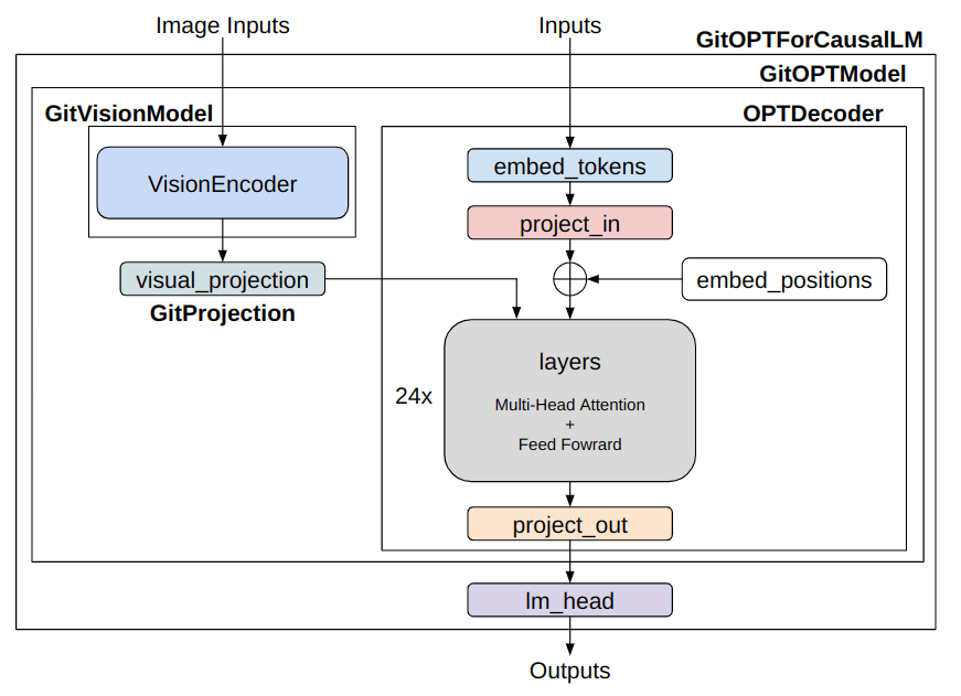
Now, let’s connect GIT and OPT. The goal is to create a model as shown in the figure.
Simplified model architecture of GIT-OPT (image made by the author)
For the general implementation, you can refer to the modeling_git.py.
The most important part is the GitOPTModel. Inside this, a vision encoder need to be connected with a LLM. I’ll explain some key components.
class GitOPTModel(OPTModel):
def __init__(self, config: OPTConfig):
super(GitOPTModel, self).__init__(config)
self.image_encoder = CLIPVisionModel.from_pretrained(config.vision_model_name)
self.visual_projection = GitProjection(config)
Inside the __init__ function, various modules are instantiated. The super initializes the OPTModel. In GIT, it is recommended to use a powerful image encoder trained with CLIP, so I have made it compatible with the ViT trained with CLIP. The GitProjection is taken from the original GIT implementation.
Let’s look inside the forward function. The implementation is based on the forward part of the OPTDecoder, with added information from the image encoder. Although it’s a bit lengthy, I’ve added comments in the code, so please follow each step.
class GitOPTModel(OPTModel):
...
def forward(
self,
input_ids: Optional[torch.Tensor] = None,
attention_mask: Optional[torch.Tensor] = None,
pixel_values: Optional[torch.Tensor] = None,
) -> BaseModelOutputWithPooling:
seq_length = input_shape[1]
# 1. Extract image features using ViT
visual_features = self.image_encoder(pixel_values).last_hidden_state
# 2. Convert features extracted by ViT into prompt-like Image Embeddings
projected_visual_features = self.visual_projection(visual_features)
# 3. Vectorize the tokens
inputs_embeds = self.decoder.embed_tokens(input_ids)
# 4. Obtain Positional Encoding
pos_embeds = self.embed_positions(attention_mask, 0)
# 5. Dimension adjustment of Text Embeddings specific to OPT
inputs_embeds = self.decoder.project_in(inputs_embeds)
# 6. Text Embeddings + Positional Encoding
embedding_output = inputs_embeds + pos_embeds
# 7. Concatenate Image Embeddings and Text Embeddings
hidden_states = torch.cat((projected_visual_features, embedding_output), dim=1)
# 8. Create Causal Attention Mask for Text region
tgt_mask = self._generate_future_mask(
seq_length, embedding_output.dtype, embedding_output.device
)
# 9. Create Attention Mask for GIT
combined_attention_mask = self.create_attention_mask(
tgt=embedding_output,
memory=projected_visual_features,
tgt_mask=tgt_mask,
past_key_values_length=0,
)
# 10. Pass through the Decoder layer repeatedly, the main part of the language model
for idx, decoder_layer in enumerate(self.decoder.layers):
layer_outputs = decoder_layer(
hidden_states,
attention_mask=combined_attention_mask,
output_attentions=output_attentions,
use_cache=use_cache,
)
hidden_states = layer_outputs[0]
# 11. Dimension adjustment MLP specific to OPT
hidden_states = self.decoder.project_out(hidden_states)
# 12. Align the output interface
return BaseModelOutputWithPast(
last_hidden_state=hidden_states,
past_key_values=next_cache,
hidden_states=all_hidden_states,
attentions=all_self_attns,
)
Although it might look complicated, if you go through each step, you’ll see that it follows the flow illustrated in the diagram. The actual code may look a bit more complex, but grasping the main process first will make understanding the other parts easier. This is pseudocode, so for detailed parts, please refer to the published implementation.
Finally, let’s take a brief look at the GITOPTForCausalLM part.
class GitOPTForCausalLM(OPTForCausalLM):
def __init__(
self,
config,
):
super(GitOPTForCausalLM, self).__init__(config)
self.model = GitOPTModel(config)
def forward(
...
) -> CausalLMOutputWithPast:
outputs = self.model(
...
)
sequence_output = outputs[0]
logits = self.lm_head(sequence_output)
loss = None
if labels is not None:
# Predict the next word as the task
num_image_tokens = self.image_patch_tokens
shifted_logits = logits[:, num_image_tokens:-1, :].contiguous()
labels = labels[:, 1:].contiguous()
loss_fct = CrossEntropyLoss()
loss = loss_fct(shifted_logits.view(-1, self.config.vocab_size), labels.view(-1))
return CausalLMOutputWithPast(
loss=loss,
logits=logits,
...
)
The processing inside the model is simple. When labels are provided, i.e., during training, the loss calculation is also performed within the forward. In shifted_logits, tokens were fetched from the first token to the second-to-last token of the text tokens. It then calculates the Cross Entropy Loss with the labels shifted by one word as the correct answer.
One thing to note is to name the variable that assigns the GitOPTModel in the initialization function as self.model. If you check the implementation of the parent class OPTForCausalLM, you'll see that OPT is first placed to self.model during the super initialization. If you change this instance variable name, you will end up holding two OPTs, which can strain the memory.
LoRA Extension
In order to fine-tune the LLM effectively, I’ll use a library called Parameter-Efficient Fine-Tuning (PEFT). As it’s developed by Hugging Face, it integrates seamlessly with Transfors. While there are various methods within PEFT, this time I’m going to do some experiments using a commonly seen approach called Low-rank adaptation (LoRA).
Models can be applied LoRA in just a few lines if the models support PEFT.
from transformers import AutoModelForCausalLM
from peft import get_peft_config, get_peft_model, LoraConfig
model = AutoModelForCausalLM.from_pretrained('microsoft/git-base')
peft_config = LoraConfig(
task_type="CAUSAL_LM",
r=8,
lora_alpha=32,
lora_dropout=0.1,
target_modules=["v_proj"]
)
peft_model = get_peft_model(model, peft_config)
The target_modules argument specifies which modules you want to convert to LoRA. If a list is provided as target_modules, it is implemented to convert to LoRA for modules that end with each of the strings. LoRA is applied only to “value” (v_proj) of the self attention module for simplicity.
In the model, ViT is used for the image encoder part. Be cautious, as specifying it like this, self attention part of ViT might also be applied LoRA. It’s a bit tedious, but by specifying down to the part where the key names don’t overlap and giving it to target_modules, you can avoid this.
target_modules = [f"model.image_encoder.vision_model.encoder.{i}.self_attn.v_proj" for i in range(len(model.model.decoder))]
The resulting model becomes an instance of the PeftModelForCausalLM class. It has an instance variable named base_model that holds the original model converted to LoRA. As an example, I show that LoRA is applied to v_proj of the self attention in ViT.
(self_attn): GitVisionAttention(
(k_proj): Linear(in_features=768, out_features=768, bias=True)
(v_proj): Linear(
in_features=768, out_features=768, bias=True
(lora_dropout): ModuleDict(
(default): Dropout(p=0.1, inplace=False)
)
(lora_A): ModuleDict(
(default): Linear(in_features=768, out_features=8, bias=False)
)
(lora_B): ModuleDict(
(default): Linear(in_features=8, out_features=768, bias=False)
)
(lora_embedding_A): ParameterDict()
(lora_embedding_B): ParameterDict()
)
(q_proj): Linear(in_features=768, out_features=768, bias=True)
(out_proj): Linear(in_features=768, out_features=768, bias=True)
)
Inside the v_proj Linear, you'll find added fully connected layers such as lora_A and lora_B. The LoRA-converted Linear module is a namesake Linear class that inherits from PyTorch's Linear and LoraLayer. It's a somewhat unique module, so those curious about the details should take a look at the implementation.
Note that models created with PEFT will not save anything other than the LoRA part by default. While there’s a method to save using the merge_and_unload method, you might want to save all models being saved midway during training with Trainer. Overloading the Trainer's _save_checkpoints method is one approach, but to avoid the hassle, I handled it this time by fetching just the original model part held inside the PeftModel during the training phase.
model = get_peft_model(model, peft_config)
model.base_model.model.lm_head = model.lm_head
model = model.base_model.model
I believe there are more efficient ways to handle this, so I’m still researching.
Experimenting with GIT-LLM
Let’s now conduct some experiments using the model developed so far.
For details on the training configuration and other setups, please refer to the published implementation, as they essentially follow the same method.
Dataset: M3IT
For experiments, I wanted to use a dataset that pairs images with text and is easy to integrate. While exploring the Hugging face’s Datasets, I came across M3IT, a multimodal dataset for Instruction Tuning developed by the Shanghai AI Lab. Instruction Tuning is a method that yields impressive results even with a limited amount of data. It appears that M3IT has re-annotated various existing datasets specifically for Instruction Tuning.
https://huggingface.co/datasets/MMInstruction/M3IT
This dataset is easy to use, so I’ve decided to utilize it for the following experiments.
To train using M3IT, it’s necessary to create a custom Pytorch Dataset.
class SupervisedDataset(Dataset):
def __init__(
self,
vision_model_name: str,
model_name: str,
loaded_dataset: datasets.GeneratorBasedBuilder,
max_length: int = 128,
):
super(SupervisedDataset, self).__init__()
self.loaded_dataset = loaded_dataset
self.max_length = max_length
self.processor = AutoProcessor.from_pretrained("microsoft/git-base")
# Setting up the corresponding Processor for each model
self.processor.image_processor = CLIPImageProcessor.from_pretrained(vision_model_name)
self.processor.tokenizer = AutoTokenizer.from_pretrained(
model_name, padding_side="right", use_fast=False
)
def __len__(self) -> int:
return len(self.loaded_dataset)
def __getitem__(self, index) -> dict:
# cf: https://huggingface.co/datasets/MMInstruction/M3IT#data-instances
row = self.loaded_dataset[index]
# Creating text input
text = f'##Instruction: {row["instruction"]} ##Question: {row["inputs"]} ##Answer: {row["outputs"]}'
# Loading the image
image_base64_str_list = row["image_base64_str"] # str (base64)
img = Image.open(BytesIO(b64decode(image_base64_str_list[0])))
inputs = self.processor(
text,
img,
return_tensors="pt",
max_length=self.max_length,
padding="max_length",
truncation=True,
)
# batch size 1 -> unbatch
inputs = {k: v[0] for k, v in inputs.items()}
inputs["labels"] = inputs["input_ids"]
return inputs
In the __init__ function, the image_processor and tokenizer correspond to their respective models. The loaded_dataset argument passed should be from MMInstruction/M3IT datasets.
coco_datasets = datasets.load_dataset("MMInstruction/M3IT", "coco")
test_dataset = coco_datasets["test"]
For the COCO Instruction Tuning dataset, the split between training, validation, and testing is identical to the original dataset, with 566,747, 25,010, and 25,010 image-text pairs respectively. Other datasets, such as VQA or Video, can also be handled similarly, making it a versatile dataset for validation purposes.
A sample data looks like this:
Image is cited from data in M3IT.
The caption for this picture is as follows:
##Instruction: Write a succinct description of the image, capturing its main components, the relationships between them, and any notable details. ##Question: ##Answer: A man with a red helmet on a small moped on a dirt road.
For the COCO dataset, which is for Captions, the Question portion is left blank.
Let’s delve deeper into the processor’s operations. Essentially, it normalizes images and tokenizes text. Inputs shorter than max_length are also padded. The processed data returned by the processor is a dictionary containing:
- input_ids: An array of tokenized text.
- attention_mask: A mask for tokenized text (with Padding being 0).
- pixel_values: An array of normalized images, also converted to Channel-first.
These key names correspond to the arguments for the model’s forward function, so they shouldn’t be altered. Finally, input_ids are directly passed to a key named labels. The forward function of GitOPTForCausalLM calculates the loss by predicting the next word shifted by one token.
Experiment 1: Determining Fine-tuning Locations
In the research papers on GIT models, it was explained that a strong vision encoder is utilized and random parameters are adopted for the language model. This time, since the goal is to ultimately use a 7B-class language model, a pre-trained model will be applied to the language model. The following modules will be examined for fine-tuning. The GIT Projection, being an initialized module, is always included. Some combinations may seem redundant, but they are explored without too much concern for this trial.
Modules set for training are given gradients, while the rest are modified to not have gradients.
# Specifying the parameters to train (training all would increase memory usage)
for name, p in model.model.named_parameters():
if np.any([k in name for k in keys_finetune]):
p.requires_grad = True
else:
p.requires_grad = False
The Vision Encoder and LLM used for this examination are:
- openai/clip-vit-base-patch16
- facebook/opt-350m
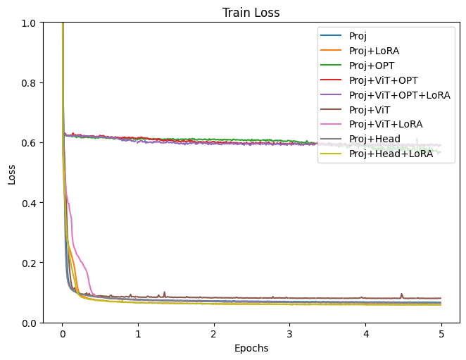
Training utilizes COCO dataset and lasts for 5 epochs.
Here are the target modules trained during each experiment:
- Proj: GIT Projection. Initialized randomly, so it’s always trained.
- LoRA: Query, Key, and Value of the self attention in the language model were applid.
- OPT: All layers were trained.
- ViT: All layers were trained.
- Head: The final lm_head of OPT was trained.
(Note: While LoRA can be applied to ViT, but to avoid making the experiments too complicated, it wasn’t included this time.)
This figure shows training loss. Proj, LoRA, OPT, ViT, and Head in the legend are the trained modules explained above. (figure made by the author)
As shown in the training loss plot, it’s apparent that some groups are not performing well. These were the case when OPT is included in the training. Although all experiments were conducted under fairly similar conditions, more detailed adjustments, such as learning rate, might be necessary when fine-tuning the language model. Results, excluding the models where OPT is included in training, will be examined next.
This figure shows training loss without full finetuning results. Proj, LoRA, OPT, ViT, and Head in the legend are the trained modules explained above. (figure made by the author)
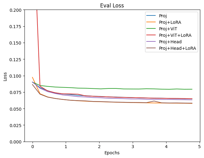
This figure shows validation loss. Proj, LoRA, OPT, ViT, and Head in the legend are the trained modules explained above. (figure made by the author)
Both training and validation Loss decreased most with the Projection+LoRA model. Fine-tuning final Head layer showed nearly identical outcomes. If ViT is also trained, the Loss appears slightly higher and results seem unstable. Even when adding LoRA during ViT training, the loss still tends to be high. For fine-tuning with this data, it seems using a pre-trained ViT model without updating its parameters yields more stable results. The effectiveness of LoRA has been acknowledged in various places, and it is evident from this experiment that adding LoRA to the LLM improved bothe traininng and validation loss.
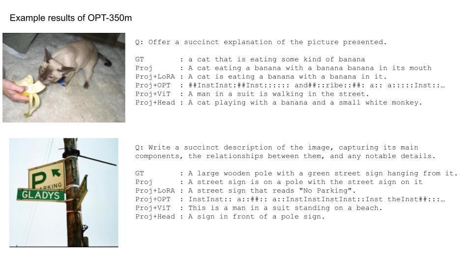
Reviewing the inference results on some test data:
Example results of GIT-OPT. Pictures are cited from M3IT dataset, and text results were made by the author’s model
When training OPT itself, the results are as poor as the result of loss, making the model at a loss for words. Additionally, when training ViT, the output makes semantic sense, but describes something entirely different from the given image. However, the other results seem to capture the features of the images to some extent. For instance, the first image mentions “cat” and “banana”, and the second one identifies “traffic sign”. Comparing results with and without LoRA, the latter tends to repetitively use similar words, but using LoRA seems to make it slightly more natural. Training the Head results in intriguing outputs, like using “playing” instead of “eating” for the first image. While there are some unnatural elements in these results, it can be deduced that the training was successful in capturing image features.
Experiment 2: Comparing Billion-Scale Models
For fine-tuning conditions in earlier experiments, a slightly smaller language model, OPT-350m, was used. Now, the intention is to switch the language model to a 7B model. Not just settling for OPT, stronger LLMs, LLaMA and MPT, will also be introduced.
Integrating these two models can be done in a similar fashion to OPT. Referring to the forward functions of the LlamaModel and MPTModel, combine the projected image vectors with text tokens, and change the mask from Causal Attention Mask to GIT’s Attention Mask. One thing to note: for MPT, the mask isn’t (0, -inf), but (False, True). The subsequent processes can be implemented similarly.
To use the 7B-class model with OPT, merely change the model name from facebook/opt-350m to facebook/opt-6.7b.
For LLaMA, with the availability of LLaMA2, that will be the model of choice. To use this pre-trained model, approvals from both Meta and Hugging Face are needed. An account is necessary for Hugging Face, so make sure to set that up. Approvals typically come within a few hours. Afterwards, log into Hugging Face on the terminal where training is executed.
huggingface-cli login
You can log in using the token created in Hugging Face account → Settings → Access Token.
Training parameters remain consistent, using the COCO dataset and lasting for 3 epochs. Based on results from Experiment 1, the modules set for fine-tuning were Projection + LoRA.
Let’s take a look at the results.
This figure shows training loss (figure made by the author)
This figure shows validation loss (figure made by the author)
Reviewing the loss, it’s apparent that the models using LLaMA2 and MPT as LLM show a more satisfactory reduction. Let’s also observe the inference results.
Example results of GIT-LLMs. Pictures are cited from M3IT dataset, and text results were made by the author’s model
Regarding the first image, for all models, the expressions seem more natural compared to OPT-350m. There are no bizarre expressions like “a banana with a banana”, highlighting the strength of LLM. For the second image, there’s still some difficulty with phrases like “a traffic light” or “a building”. For such complex images, there might be a need to consider upgrading the ViT model.
Finally, let’s run inference on images that became popular with GPT-4.
Example results of GIT-LLMs. A picture is cited from here, and text results were made by the author’s models
Although fluent responses were anticipated since LLM is in use, the outcomes are quite simple. This might be because the model was trained solely on COCO.
Experiment 3. Increasing the Data
Given the underwhelming results of the previous experiment, it was decided to incorporate data other than COCO for training. The M3IT dataset currently in use is quite comprehensive, and it can handle a significant amount of data in the same format as COCO.
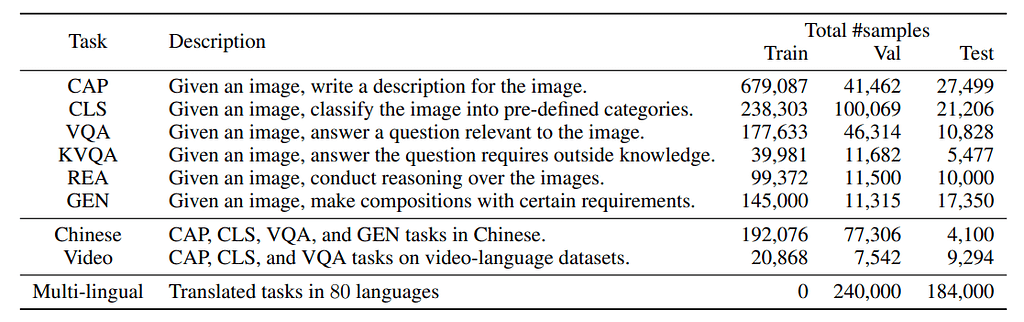
This table is cited from Table 3 of “M3IT: A Large-Scale Dataset towards Multi-Modal Multilingual Instruction Tuning”
It is intended to use data from this source excluding the “Chinese” and “Video” categories. Originally, the COCO training dataset contained 566,747 pieces of data. By combining it with additional sources, this increased to 1,361,650. Although the size has roughly doubled, the dataset is believed to have become of higher quality due to the increased diversity of tasks.
Handling multiple Pytorch datasets can be easily achieved using the ConcatDataset.
dataset_list = [
datasets.load_dataset("MMInstruction/M3IT", i) for i in m3it_name_list
]
train_dataset = torch.utils.data.ConcatDataset([d["train"] for d in dataset_list])
The training was conducted for 1 epoch, and the LLaMA2 model was used for fine-tuning the Projection and LoRA, similarly to Experiment 2.
As there’s no loss to compare to this time, let’s dive straight into the inference results.
Example results of GIT-LLaMA2. Pictures are cited from M3IT dataset, and text results were made by the author’s model
Example results of GIT-LLaMA2. Pictures are cited from M3IT dataset, and text results were made by the author’s model
Example results of GIT-LLaMA2. Pictures are cited from M3IT dataset, and text results were made by the author’s model
Along with solving simple problems, the model now handles more complex challenges. By adding datasets for tasks more intricate than just captioning, the capabilities have expanded significantly. Achieving this level of accuracy with only 1 epoch of training was surprising.
Let’s test it with the following example image. Given the increased variety in the dataset, the way the questions were presented was slightly modified.
Example results of GIT-LLaMA2. A picture is cited from here, and text results were made by the author’s models
While the description being “Umbrella” was still wired, it feels like it’s getting better. To improve further, there’s a need to increase the number of training epochs, add more types or volumes of datasets, and leverage more powerful ViT or LLM. Nonetheless, it’s impressive that such a model could be developed in just half a day given the computational and data resources.
Bonus Experiment. Did the Image Turn into Words?
Let’s take another look at the GIT structure.
Simplified model architecture of GIT-LLM (image made by the author)
As shown in the figure, after feature extraction by the vision encoder, images are treated on par with vectorized text through Visual Projection. In other words, it’s possible that the Visual Projection is converting image vectors into text vectors. An investigation was conducted to see what the vectors look like after theVisual Projection.
While there’s an option to use the Head to revert the vector post-projection back to text, it was found that even vectors that were vectorized using the Embedding module could not be reverted back to their original text using this method. Therefore, vectors that closely resemble the text vectors before being input into the LLM should be assigned as the corresponding word. All tokens registered in the tokenizer were vectorized using the Embedding module, and the one with the highest cosine similarity was identified as the target word.
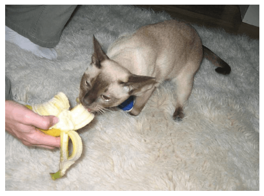
The image used for this experiment is that of a cat.
A Picture is cited from M3IT dataset.
Now, let’s proceed with the analysis (whole analysis is available here). First, all the registered tokens are vectorized.
coco_datasets = datasets.load_dataset("MMInstruction/M3IT", "coco")
test_dataset = coco_datasets["test"]
supervised_test_dataset = SupervisedDataset(model_name, vision_model_name, test_dataset, 256)
ids = range(supervised_test_dataset.processor.tokenizer.vocab_size)
all_ids = torch.tensor([i for i in ids]).cuda()
token_id_to_features = model.model.embed_tokens(all_ids)
Next, the image vectors that would have been converted to words by the ViT and Projection are extracted.
inputs = supervised_test_dataset[0] # Picking a sample arbitrarily
pixel_values = inputs["pixel_values"]
out_vit = model.model.image_encoder(pixel_values).last_hidden_state
out_vit = model.model.visual_projection(out_vit)
The dot products of these vectors and the word vectors were calculated, and the results with the maximum value were decoded as the relevant token ID.
# Dot product
nearest_token = out_vit[0] @ token_id_to_features.T
# The index of the maximum value corresponds to the relevant token ID
visual_out = nearest_token.argmax(-1).cpu().numpy()
decoded_text = supervised_test_dataset.processor.tokenizer.batch_decode(visual_out)
print(decoded_text)
"""
['otr', 'eg', 'anto', 'rix', 'Nas', ...]
"""
As shown in the printed decoded_text, some unfamiliar words have appeared. As some words are repeated, they were counted.
print(pd.Series(decoded_text).value_counts())
"""
mess 43
atura 29
せ 10
Branch 10
Enum 9
bell 9
worden 7
...
"""
A large number of unfamiliar words seem to have appeared. Depending on the position, they might convey meaningful information. Let’s plot the words against the cat image.
n_patches = 14
IMAGE_HEIGHT = 468
IMAGE_WIDTH = 640
y_list = np.arange(15, IMAGE_HEIGHT, IMAGE_HEIGHT//n_patches)
x_list = np.arange(10, IMAGE_WIDTH, IMAGE_WIDTH//n_patches)
plt.figure()
plt.axis("off")
plt.imshow(np.array(image), alpha=0.4)
for index in np.arange(n_patches ** 2):
y_pos = index // n_patches
x_pos = index - y_pos * n_patches
y = y_list[y_pos]
x = x_list[x_pos]
# The first token is the bos token, so it is excluded
word = decoded_text[index + 1]
# For differentiating words by color
plt.annotate(word, (x, y), size=7, color="blue")
plt.show()
plt.clf()
plt.close()
Image made by the author
Words that frequently appear are color-coded. The result seems to suggest that they are not simply being projected onto meaningful words. While the word “Cat” might be superimposed on the cat image, giving it some relevance, its meaning remains unclear.
The inconclusive results in this experiment might be due to forcibly selecting a word with a high cosine similarity. At any rate, the approach doesn’t involve simply casting words and creating image prompts. Vectors extracted from images are converted by Visual Projection into vectors in token space, which seem to hold some resemblance in meaning, functioning as mysterious prompts. It might be best not to delve any deeper into this.
Conclusion
In this tech blog post, I introduced the method of integrating LLMs into the vision language model, GIT. Furthermore, various experiments were conducted using the developed models. While there were successes and failures, I would like to continue conducting experiments with vision language models to accumulate insights. Please consider this article as a reference and feel encouraged to create your own vision language models and explore its potential.
This is an illustrated image of GIT-LLM created using Stable Diffusion. (Image made by the author)
Build and Play! Your Own V&L Model Equipped with LLM! was originally published in Towards Data Science on Medium, where people are continuing the conversation by highlighting and responding to this story.