Using PyTorch, computer vision techniques, and a Convolutional Neural Network (CNN), I worked on a model that tracks players, teams and basic performance statistics
Nowadays, I don’t play hockey as much as I want to, but it’s been a part of me since I was a kid. Recently, I had the chance to help with the referee table and keep some stats in the first Ice Hockey Tournament in Lima (3 on 3). This event involved an extraordinary effort of the the Peruvian Inline Hockey Association (APHL) and a kind visit from the Friendship League. To add an AI twist, I used PyTorch, computer vision techniques, and a Convolutional Neural Network (CNN) to build a model that tracks players and teams and gathers some basic performance stats.
This article aims to be a quick guide to designing and deploying the model. Although the model still needs some fine-tuning, I hope it can help anyone introduce themselves to the interesting world of computer vision applied to sports. I would like to acknowledge and thank the Peruvian Inline Hockey Association (APHL) for allowing me to use a 40-second video sample of the tournament for this project (you can find the video input sample in the project’s GitHub repository).
The Architecture
Before moving on with the project, I did some quick research to find a baseline from which I could work and avoid “reinventing the wheel”. I found that in terms of using computer vision to track players, there is a lot of interesting work on football (not surprising, being the most popular team sport in the world). However, I didn’t find many resources for ice hockey. Roboflow has some interesting pre-trained models and datasets for training your own, but working with a hosted model presented some latency issues that I will explain further. In the end, I leveraged the soccer material for reading the video frames and obtaining the individual track IDs, following the basic principles and tracking method approach explained in this tutorial (If you are interested in gaining a better understanding of some basic computer vision techniques, I suggest watching at least the first hour and a half of the tutorial).
With the tracking IDs covered, I then built my own path. As we walk through this article, we’ll see how the project evolves from a simple object detection task to a model that fully detects players, teams, and delivers some basic performance metrics (sample clips from 01 to 08, author’s own creation).
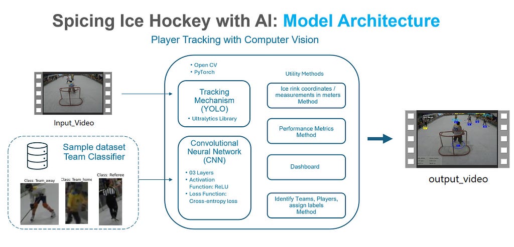
Model Architecture. Author’s own creation
The Tracking Mechanism
The tracking mechanism is the backbone of the model. It ensures that each detected object within the video is identified and assigned a unique identifier, maintaining this identity across each frame. The main components of the tracking mechanism are:
- YOLO (You Only Look Once): It’s a powerful real-time object detection algorithm originally introduced in 2015 in the paper “You Only Look Once: Unified, Real-Time Object Detection”. Stands out for its speed and its versatility in detecting around 80 pre-trained classes (it’s important to note that it can also be trained on custom datasets to detect specific objects). For our use case, we will rely on YOLOv8x, a computer vision model built by Ultralytics based on previous YOLO versions. You can download it here.
- ByteTrack Tracker: To understand ByteTrack, we have to understand MOT (Multiple Object Tracking), which involves tracking the movements of multiple objects over time in a video sequence and linking those objects detected in a current frame with corresponding objects in previous frames. To accomplish this, we will use ByteTrack ( introduced in 2021 in the paper “ByteTrack: Multi-Object Tracking by Associating Every Detection Box”). To implement the ByteTrack tracker and assign track IDs to detected objects, we will rely on the Python’s supervision library.
- OpenCV: is a well-known library for various computer vision tasks in Python. For our use case, we will rely on OpenCV to visualize and annotate video frames with bounding boxes and text for each detected object.
In order to build our tracking mechanism, we’ll begin with these initial two steps:
- Deploying the YOLO model with ByteTrack to detect objects (in our case, players) and assign unique track IDs.
- Initializing a dictionary to store object tracks in a pickle (pkl) file. This will be extremely useful to avoid executing the video frame-by-frame object detection process each time we run the code, and save significant time.
For the following step, these are the Python packages that we’ll need:
pip install ultralytics
pip install supervision
pip install opencv-python
Next, we’ll specify our libraries and the path for our sample video file and pickle file (if it exists; if not, the code will create one and save it in the same path):
#**********************************LIBRARIES*********************************#
from ultralytics import YOLO
import supervision as sv
import pickle
import os
import cv2
# INPUT-video file
video_path = 'D:/PYTHON/video_input.mp4'
# OUTPUT-Video File
output_video_path = 'D:/PYTHON/output_video.mp4'
# PICKLE FILE (IF AVAILABLE LOADS IT IF NOT, SAVES IT IN THIS PATH)
pickle_path = 'D:/PYTHON/stubs/track_stubs.pkl'
Now let’s go ahead and define our tracking mechanism (you can find the video input sample in the project’s GitHub repository):
#*********************************TRACKING MECHANISM**************************#
class HockeyAnalyzer:
def __init__(self, model_path):
self.model = YOLO(model_path)
self.tracker = sv.ByteTrack()
def detect_frames(self, frames):
batch_size = 20
detections = []
for i in range(0, len(frames), batch_size):
detections_batch = self.model.predict(frames[i:i+batch_size], conf=0.1)
detections += detections_batch
return detections
#********LOAD TRACKS FROM FILE OR DETECT OBJECTS-SAVES PICKLE FILE************#
def get_object_tracks(self, frames, read_from_stub=False, stub_path=None):
if read_from_stub and stub_path is not None and os.path.exists(stub_path):
with open(stub_path, 'rb') as f:
tracks = pickle.load(f)
return tracks
detections = self.detect_frames(frames)
tracks = {"person": []}
for frame_num, detection in enumerate(detections):
cls_names = detection.names
cls_names_inv = {v: k for k, v in cls_names.items()}
# Tracking Mechanism
detection_supervision = sv.Detections.from_ultralytics(detection)
detection_with_tracks = self.tracker.update_with_detections(detection_supervision)
tracks["person"].append({})
for frame_detection in detection_with_tracks:
bbox = frame_detection[0].tolist()
cls_id = frame_detection[3]
track_id = frame_detection[4]
if cls_id == cls_names_inv.get('person', None):
tracks["person"][frame_num][track_id] = {"bbox": bbox}
for frame_detection in detection_supervision:
bbox = frame_detection[0].tolist()
cls_id = frame_detection[3]
if stub_path is not None:
with open(stub_path, 'wb') as f:
pickle.dump(tracks, f)
return tracks
#***********************BOUNDING BOXES AND TRACK-IDs**************************#
def draw_annotations(self, video_frames, tracks):
output_video_frames = []
for frame_num, frame in enumerate(video_frames):
frame = frame.copy()
player_dict = tracks["person"][frame_num]
# Draw Players
for track_id, player in player_dict.items():
color = player.get("team_color", (0, 0, 255))
bbox = player["bbox"]
x1, y1, x2, y2 = map(int, bbox)
# Bounding boxes
cv2.rectangle(frame, (x1, y1), (x2, y2), color, 2)
# Track_id
cv2.putText(frame, str(track_id), (x1, y1 - 10), cv2.FONT_HERSHEY_SIMPLEX, 0.9, color, 2)
output_video_frames.append(frame)
return output_video_frames
The method begins by initializing the YOLO model and the ByteTrack tracker. Next, each frame is processed in batches of 20, using the YOLO model to detect and collect objects in each batch. If the pickle file is available in its path, it precomputes the tracks from the file. If the pickle file is not available (you are running the code for the first time or have erased a previous pickle file), the get_object_tracks converts each detection into the required format for ByteTrack, updates the tracker with these detections, and stores the tracking information in a new pickle file in the designated path.Finally, iterations are made over each frame, drawing bounding boxes and track IDs for each detected object.
To execute the tracker and save a new output video with bounding boxes and track IDs, you can use the following code:
#*************** EXECUTES TRACKING MECHANISM AND OUTPUT VIDEO****************#
# Read the video frames
video_frames = []
cap = cv2.VideoCapture(video_path)
while cap.isOpened():
ret, frame = cap.read()
if not ret:
break
video_frames.append(frame)
cap.release()
#********************* EXECUTE TRACKING METHOD WITH YOLO**********************#
tracker = HockeyAnalyzer('D:/PYTHON/yolov8x.pt')
tracks = tracker.get_object_tracks(video_frames, read_from_stub=True, stub_path=pickle_path)
annotated_frames = tracker.draw_annotations(video_frames, tracks)
#*********************** SAVES VIDEO FILE ************************************#
fourcc = cv2.VideoWriter_fourcc(*'mp4v')
height, width, _ = annotated_frames[0].shape
out = cv2.VideoWriter(output_video_path, fourcc, 30, (width, height))
for frame in annotated_frames:
out.write(frame)
out.release()
If everything in your code worked correctly, you should expect a video output similar to the one shown in sample clip 01.
Sample Clip 01: Basic tracking mechanism ( Objects and Tracking IDs)
TIP #01: Don’t underestimate your compute power! When running the code for the first time, expect the frame processing to take some time, depending on your compute capacity. For me, it took between 45 to 50 minutes using only a CPU setup (consider CUDA as an option). The YOLOv8x tracking mechanism, while powerful, demands significant compute resources (at times, my memory hit 99%, fingers crossed it didn’t crash!🙄). If you encounter issues with this version of YOLO, lighter models are available on Ultralytics’ GitHub to balance accuracy and compute capacity.
The Ice RinkAs you’ve seen from the first step, we have some challenges. Firstly, as expected, the model picks up all moving objects; players, referees, even those outside the rink. Secondly, those red bounding boxes can make tracking players a bit unclear and not very neat for presentation. In this section, we’ll focus on narrowing our detection to objects within the rink only. Plus, we’ll swap out those bounding boxes for ellipses at the bottom, ensuring clearer visibility.
Let’s switch from using boxes to using ellipses first. To accomplish this, we’ll simply add a new method above the labels and bounding boxes method in our existing code:
#************ Design of Ellipse for tracking players instead of Bounding boxes**************#
def draw_ellipse(self, frame, bbox, color, track_id=None, team=None):
y2 = int(bbox[3])
x_center = (int(bbox[0]) + int(bbox[2])) // 2
width = int(bbox[2]) - int(bbox[0])
color = (255, 0, 0)
text_color = (255, 255, 255)
cv2.ellipse(
frame,
center=(x_center, y2),
axes=(int(width) // 2, int(0.35 * width)),
angle=0.0,
startAngle=-45,
endAngle=235,
color=color,
thickness=2,
lineType=cv2.LINE_4
)
if track_id is not None:
rectangle_width = 40
rectangle_height = 20
x1_rect = x_center - rectangle_width // 2
x2_rect = x_center + rectangle_width // 2
y1_rect = (y2 - rectangle_height // 2) + 15
y2_rect = (y2 + rectangle_height // 2) + 15
cv2.rectangle(frame,
(int(x1_rect), int(y1_rect)),
(int(x2_rect), int(y2_rect)),
color,
cv2.FILLED)
x1_text = x1_rect + 12
if track_id > 99:
x1_text -= 10
font_scale = 0.4
cv2.putText(
frame,
f"{track_id}",
(int(x1_text), int(y1_rect + 15)),
cv2.FONT_HERSHEY_SIMPLEX,
font_scale,
text_color,
thickness=2
)
return frame
We’ll also need to update the annotation step by replacing the bounding boxes and IDs with a call to the ellipse method:
#***********************BOUNDING BOXES AND TRACK-IDs**************************#
def draw_annotations(self, video_frames, tracks):
output_video_frames = []
for frame_num, frame in enumerate(video_frames):
frame = frame.copy()
player_dict = tracks["person"][frame_num]
# Draw Players
for track_id, player in player_dict.items():
bbox = player["bbox"]
# Draw ellipse and tracking IDs
self.draw_ellipse(frame, bbox, (0, 255, 0), track_id)
x1, y1, x2, y2 = map(int, bbox)
output_video_frames.append(frame)
return output_video_frames
With these changes, your output video should look much neater, as shown in sample clip 02.
Sample Clip 02: Replacing bounding boxes with ellipses
Now, to work with the rink boundaries, we need to have some basic knowledge of resolution in computer vision. In our use case, we are working with a 720p (1280x720 pixels) format, which means that each frame or image we process has dimensions of 1280 pixels (width) by 720 pixels (height).
What does it mean to work with a 720p (1280x720 pixels) format? It means that the image is made up of 1280 pixels horizontally and 720 pixels vertically. Coordinates in this format start at (0, 0) in the top-left corner of the image, with the x-coordinate increasing as you move right and the y-coordinate increasing as you move down. These coordinates are used to mark specific areas in the image, like using (x1, y1) for the top-left corner and (x2, y2) for the bottom-right corner of a box. Understanding this will helps us measure distances and speeds, and decide where in the video we want to focus our analysis.
That said, we will start marking the frame borders with green lines using the following code:
#********************* Border Definition for Frame***********************
import cv2
video_path = 'D:/PYTHON/video_input.mp4'
cap = cv2.VideoCapture(video_path)
#**************Read, Define and Draw corners of the frame****************
ret, frame = cap.read()
bottom_left = (0, 720)
bottom_right = (1280, 720)
upper_left = (0, 0)
upper_right = (1280, 0)
cv2.line(frame, bottom_left, bottom_right, (0, 255, 0), 2)
cv2.line(frame, bottom_left, upper_left, (0, 255, 0), 2)
cv2.line(frame, bottom_right, upper_right, (0, 255, 0), 2)
cv2.line(frame, upper_left, upper_right, (0, 255, 0), 2)
#*******************Save the frame with marked corners*********************
output_image_path = 'rink_area_marked_VALIDATION.png'
cv2.imwrite(output_image_path, frame)
print("Rink area saved:", output_image_path)
The result should be a green rectangle as shown in (a) in sample clip 03. But in order to track only the moving objects within the rink we would need a delimitation more similar to the one in (b) .
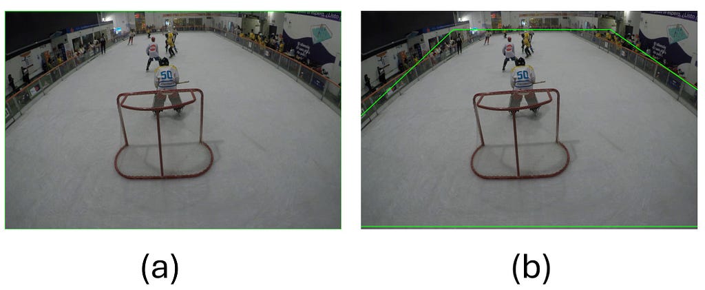
Figure 03: Border Definition for the Ice Rink (Author’s own creation)
Getting (b) right is like an iterative process of trial and error, where you test different coordinates until you find the boundaries that best fit your model. Initially, I aimed to match the rink borders exactly. However, the tracking system struggled near the edges. To improve accuracy, I expanded the boundaries slightly to ensure all tracking objects within the rink were captured while excluding those outside. The outcome, shown in (b), was the best I could get (you could still work better scenarios) defined by these coordinates:
- Bottom Left Corner: (-450, 710)
- Bottom Right Corner: (2030, 710)
- Upper Left Corner: (352, 61)
- Upper Right Corner: (948, 61)
Finally, we will define two additional areas: the offensive zones for both the White and Yellow teams (where each team aims to score). This will enable us to gather some basic positional statistics and pressure metrics for each team within their opponent’s zone.
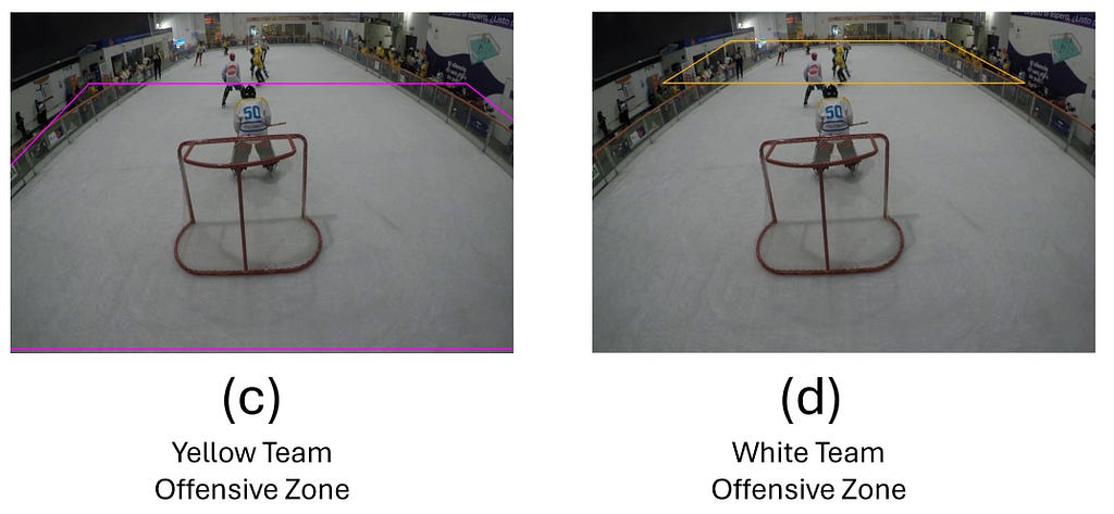
Figure 04: Offensive Zones ( Author’s own creation)
#**************YELLOW TEAM OFFENSIVE ZONE****************
Bottom Left Corner: (-450, 710)
Bottom Right Corner: (2030, 710)
Upper Left Corner: (200, 150)
Upper Right Corner: (1160, 150)
#**************WHITE TEAM OFFENSIVE ZONE****************
Bottom Left Corner: (180, 150)
Bottom Right Corner: (1100, 150)
Upper Left Corner: (352, 61)
Upper Right Corner: (900, 61)
We will set aside these coordinates for now and explain in the next step how we’ll classify each team. Then, we’ll bring it all together into our original tracking method.
Using Deep Learning for Team Prediction
Over 80 years have passed since the release of “A Logical Calculus of the Ideas Immanent in Nervous Activity”, the paper written by Warren McCulloch and Walter Pitts in 1943, which set the solid ground for early neural network research. Later, in 1957, the mathematical model of a simplified neuron (receiving inputs, applying weights to these inputs, summing them up, and outputting a binary result) inspired Frank Rosenblatt to build the Mark I. This was the first hardware implementation designed to demonstrate the concept of a perceptron, a neural network model capable of learning from data to make binary classifications. Since then, the quest to make computers think like us hasn’t slowed down. If this is your first deep dive into Neural Networks, or if you want to refresh and strengthen your knowledge, I recommend reading this series of articles by Shreya Rao as a great starting point for deep learning. Additionally, you can access my collection of stories (different contributors) that I’ve gathered here, and which you might find useful.
Why choose a Convolutional Neural Network (CNN)? Honestly, it wasn’t my first choice. Initially, I tried building a model with LandingAI, a user-friendly platform for cloud deployment and Python connection through APIs. However, latency issues appeared (over 1,000 frames to process online). Similar latency problems occurred with pre-trained models in Roboflow, despite their quality datasets and pre-trained models. Realizing the need to run it locally, I tried an MSE-based method to classify jersey colors for team and referee detection. While it sounded like the final solution, it showed low accuracy. After days of trial and error, I switched to CNNs. Among different deep learning approaches, CNNs are well-suited for object detection, unlike LSTM or RNN, which are better fit for sequential data like language transcription or translation.
Before diving into the code, let’s cover some basic concepts about its architecture:
- Sample Dataset for learning: The dataset has been classified into three classes: Referee, Team_Away (White jersey players), and Team_Home (Yellow jersey players). A sample of each class has been divided into two sets: training data and validation data. The training data will be used by the CNN in each iteration (Epoch) to “learn” patterns across multiple layers. The validation data will be used at the end of each iteration to evaluate the model’s performance and measure how well it generalizes to new data. Creating the sample dataset wasn’t too hard; it took me around 30 to 40 minutes to crop sample images from each class from the video and organize them into subdirectories. I managed to create a sample dataset of approximately 90 images that you can find in the project’s GitHub repository.
- How does the model learn?: Input data moves through each layer of the neural network, which can have one or multiple layers linked together to make predictions. Every layer uses an activation function that processes data to make predictions or introduce changes to the data. Each connection between these layers has a weight, which determines how much influence one layer’s output has on the next. The goal is to find the right combination of these weights that minimize mistakes when predicting outcomes. Through a process called backpropagation and a loss function, the model adjusts these weights to reduce errors and improve accuracy. This process repeats in what’s called an Epoch (forward pass + backpropagation), with the model getting better at making predictions in each cycle as it learns from its mistakes.
- Activation Function: As mentioned before, the activation function plays an important role in the model’s learning process. I chose ReLU (Rectified Linear Unit) because it is known for being computationally efficient and mitigating what is called the vanishing gradient problem (where networks with multiple layers may stop learning effectively). While ReLU works well, other functions like sigmoid, tanh, or swish also have their uses depending on how complex the network is.
- Epochs: Setting the right number of epochs involves experimentation. You should take into account factors such as the complexity of the dataset, the architecture of your CNN model, and computational resources. In most cases, it is best to monitor the model’s performance in each iteration and stop training when improvements become minimal to prevent overfitting. Given my small training dataset, I decided to start with 10 epochs as a baseline. However, adjustments may be necessary in other scenarios based on metric performance and validation results.
- Adam (Adaptive Moment Estimation): Ultimately, the goal is to reduce the error between predicted and true outputs. As mentioned before, backpropagation plays a key role here by adjusting and updating neural network weights to improve predictions over time. While backpropagation handles weight updates based on gradients from the loss function, the Adam algorithm enhances this process by dynamically adjusting the learning rate to gradually minimize the error or loss function. In other words, it fine-tunes how quickly the model learns.
That said in order to run our CNN model we will need the following Python packages:
pip install torch torchvision
pip install matplotlib
pip install scikit-learn
Tip-02: Ensure that PyTorch it’s installed properly. All my tools are set up in an Anaconda environment, and when I installed PyTorch, at first, it seemed that it was set up correctly. However, some issues appeared while running some libraries. Initially, I thought it was the code, but after several revisions and no success, I had to reinstall Anaconda and install PyTorch in a clean environment, and with that, problem fixed!
Next, we’ll specify our libraries and the path of our sample dataset:
# ************CONVOLUTIONAL NEURAL NETWORK-THREE CLASSES DETECTION**************************
# REFEREE
# WHITE TEAM (Team_away)
# YELLOW TEAM (Team_home)
import os
import torch
import torch.nn as nn
import torch.optim as optim
import torch.nn.functional as F
import torchvision.transforms as transforms
import torchvision.datasets as datasets
from torch.utils.data import DataLoader
from sklearn.metrics import accuracy_score, precision_score, recall_score, f1_score
import matplotlib.pyplot as plt
#Training and Validation Datasets
#Download the teams_sample_dataset file from the project's GitHub repository
data_dir = 'D:/PYTHON/teams_sample_dataset'
First, we will ensure each picture is equally sized (resize to 150x150 pixels), then convert it to a format that the code can understand (in PyTorch, input data is typically represented as Tensor objects). Finally, we will adjust the colors to make them easier for the model to work with (normalize) and set up a procedure to load the images. These steps together help prepare the pictures and organize them so the model can effectively start learning from them, avoiding deviations caused by data format.
#******************************Data transformation***********************************
transform = transforms.Compose([
transforms.Resize((150, 150)),
transforms.ToTensor(),
transforms.Normalize(mean=[0.5, 0.5, 0.5], std=[0.5, 0.5, 0.5])
])
# Load dataset
train_dataset = datasets.ImageFolder(os.path.join(data_dir, 'train'), transform=transform)
val_dataset = datasets.ImageFolder(os.path.join(data_dir, 'val'), transform=transform)
train_loader = DataLoader(train_dataset, batch_size=32, shuffle=True)
val_loader = DataLoader(val_dataset, batch_size=32, shuffle=False)
Next we’ll define our CNN’s architecture:
#********************************CNN Model Architecture**************************************
class CNNModel(nn.Module):
def __init__(self):
super(CNNModel, self).__init__()
self.conv1 = nn.Conv2d(3, 32, kernel_size=3, padding=1)
self.pool = nn.MaxPool2d(kernel_size=2, stride=2, padding=0)
self.conv2 = nn.Conv2d(32, 64, kernel_size=3, padding=1)
self.conv3 = nn.Conv2d(64, 128, kernel_size=3, padding=1)
self.fc1 = nn.Linear(128 * 18 * 18, 512)
self.dropout = nn.Dropout(0.5)
self.fc2 = nn.Linear(512, 3) #Three Classes (Referee, Team_away,Team_home)
def forward(self, x):
x = self.pool(F.relu(self.conv1(x)))
x = self.pool(F.relu(self.conv2(x)))
x = self.pool(F.relu(self.conv3(x)))
x = x.view(-1, 128 * 18 * 18)
x = F.relu(self.fc1(x))
x = self.dropout(x)
x = self.fc2(x)
return x
You will notice that our CNN model has three layers (conv1, conv2, conv3). The data begins in the convolutional layer (conv), where the activation function (ReLU) is applied. This function enables the network to learn complex patterns and relationships in the data. Following this, the pooling layer is activated. What is Max Pooling? It’s a technique that reduces the image size while retaining important features, which helps in efficient training and optimizes memory resources. This process repeats across conv1 to conv3. Finally, the data passes through fully connected layers (fc1, fc2) for final classification (or decision-making).
As the next step, we initialize our model, configure categorical cross-entropy as the loss function (commonly used for classification tasks), and designate Adam as our optimizer. As mentioned earlier, we’ll execute our model over a full cycle of 10 epochs.
#********************************CNN TRAINING**********************************************
# Model-loss function-optimizer
model = CNNModel()
criterion = nn.CrossEntropyLoss()
optimizer = optim.Adam(model.parameters(), lr=0.001)
#*********************************Training*************************************************
num_epochs = 10
train_losses, val_losses = [], []
for epoch in range(num_epochs):
model.train()
running_loss = 0.0
for inputs, labels in train_loader:
optimizer.zero_grad()
outputs = model(inputs)
labels = labels.type(torch.LongTensor)
loss = criterion(outputs, labels)
loss.backward()
optimizer.step()
running_loss += loss.item()
train_losses.append(running_loss / len(train_loader))
model.eval()
val_loss = 0.0
all_labels = []
all_preds = []
with torch.no_grad():
for inputs, labels in val_loader:
outputs = model(inputs)
labels = labels.type(torch.LongTensor)
loss = criterion(outputs, labels)
val_loss += loss.item()
_, preds = torch.max(outputs, 1)
all_labels.extend(labels.tolist())
all_preds.extend(preds.tolist())
To track performance, we will add some code to follow the training progress, print validation metrics, and plot them. Finally, we save the model as hockey_team_classifier.pth in a designated path of your choice.
#********************************METRICS & PERFORMANCE************************************
val_losses.append(val_loss / len(val_loader))
val_accuracy = accuracy_score(all_labels, all_preds)
val_precision = precision_score(all_labels, all_preds, average='macro', zero_division=1)
val_recall = recall_score(all_labels, all_preds, average='macro', zero_division=1)
val_f1 = f1_score(all_labels, all_preds, average='macro', zero_division=1)
print(f"Epoch [{epoch + 1}/{num_epochs}], "
f"Loss: {train_losses[-1]:.4f}, "
f"Val Loss: {val_losses[-1]:.4f}, "
f"Val Acc: {val_accuracy:.2%}, "
f"Val Precision: {val_precision:.4f}, "
f"Val Recall: {val_recall:.4f}, "
f"Val F1 Score: {val_f1:.4f}")
#*******************************SHOW METRICS & PERFORMANCE**********************************
plt.plot(train_losses, label='Train Loss')
plt.plot(val_losses, label='Validation Loss')
plt.legend()
plt.show()
# SAVE THE MODEL FOR THE GH_CV_track_teams CODE
torch.save(model.state_dict(), 'D:/PYTHON/hockey_team_classifier.pth')
Additionally, alongside your “pth” file, after running through all the steps described above (you can find the complete code in the project’s GitHub repository, you should expect to see an output like the following (metrics may vary slightly):
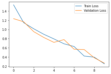
Figure 05: CNN model performance metrics
#**************CNN PERFORMANCE ACROSS TRAINING EPOCHS************************
Epoch [1/10], Loss: 1.5346, Val Loss: 1.2339, Val Acc: 47.37%, Val Precision: 0.7172, Val Recall: 0.5641, Val F1 Score: 0.4167
Epoch [2/10], Loss: 1.1473, Val Loss: 1.1664, Val Acc: 55.26%, Val Precision: 0.6965, Val Recall: 0.6296, Val F1 Score: 0.4600
Epoch [3/10], Loss: 1.0139, Val Loss: 0.9512, Val Acc: 57.89%, Val Precision: 0.6054, Val Recall: 0.6054, Val F1 Score: 0.5909
Epoch [4/10], Loss: 0.8937, Val Loss: 0.8242, Val Acc: 60.53%, Val Precision: 0.7222, Val Recall: 0.5645, Val F1 Score: 0.5538
Epoch [5/10], Loss: 0.7936, Val Loss: 0.7177, Val Acc: 63.16%, Val Precision: 0.6667, Val Recall: 0.6309, Val F1 Score: 0.6419
Epoch [6/10], Loss: 0.6871, Val Loss: 0.7782, Val Acc: 68.42%, Val Precision: 0.6936, Val Recall: 0.7128, Val F1 Score: 0.6781
Epoch [7/10], Loss: 0.6276, Val Loss: 0.5684, Val Acc: 78.95%, Val Precision: 0.8449, Val Recall: 0.7523, Val F1 Score: 0.7589
Epoch [8/10], Loss: 0.4198, Val Loss: 0.5613, Val Acc: 86.84%, Val Precision: 0.8736, Val Recall: 0.8958, Val F1 Score: 0.8653
Epoch [9/10], Loss: 0.3959, Val Loss: 0.3824, Val Acc: 92.11%, Val Precision: 0.9333, Val Recall: 0.9213, Val F1 Score: 0.9243
Epoch [10/10], Loss: 0.2509, Val Loss: 0.2651, Val Acc: 97.37%, Val Precision: 0.9762, Val Recall: 0.9792, Val F1 Score: 0.9769
After finishing 10 epochs, the CNN model shows improvement in performance metrics. Initially, in Epoch 1, the model starts with a training loss of 1.5346 and a validation accuracy of 47.37%. How should we understand this initial point?
Accuracy is one of the most common metrics for evaluating classification performance. In our case, it represents the proportion of correctly predicted classes out of the total. However, high accuracy alone doesn’t guarantee overall model performance; you still can have poor predictions for specific classes (as I experienced in early trials). Regarding training loss, it measures how effectively the model learns to map input data to the correct labels. Since we’re using a classification function, Cross-Entropy Loss quantifies the difference between predicted class probabilities and actual labels. A starting value like 1.5346 indicates significant differences between predicted and actual classes; ideally, this value should approach 0 as training progresses. As epochs progress, we observe a significant drop in training loss and an increase in validation accuracy. By the final epoch, the training and validation loss reach lows of 0.2509 and 0.2651, respectively.
To test our CNN model, we can select a sample of player images and evaluate its prediction capability. For testing, you can run the following code and utilize the validation_dataset folder in the project’s GitHub repository.
# *************TEST CNN MODEL WITH SAMPLE DATASET***************************
import os
import torch
import torch.nn as nn
import torch.nn.functional as F
import torchvision.transforms as transforms
from PIL import Image
# SAMPLE DATASET FOR VALIDATION
test_dir = 'D:/PYTHON/validation_dataset'
# CNN MODEL FOR TEAM PREDICTIONS
class CNNModel(nn.Module):
def __init__(self):
super(CNNModel, self).__init__()
self.conv1 = nn.Conv2d(3, 32, kernel_size=3, padding=1)
self.pool = nn.MaxPool2d(kernel_size=2, stride=2, padding=0)
self.conv2 = nn.Conv2d(32, 64, kernel_size=3, padding=1)
self.conv3 = nn.Conv2d(64, 128, kernel_size=3, padding=1)
self.fc1 = nn.Linear(128 * 18 * 18, 512)
self.dropout = nn.Dropout(0.5)
self.fc2 = nn.Linear(512, 3)
def forward(self, x):
x = self.pool(F.relu(self.conv1(x)))
x = self.pool(F.relu(self.conv2(x)))
x = self.pool(F.relu(self.conv3(x)))
x = x.view(-1, 128 * 18 * 18)
x = F.relu(self.fc1(x))
x = self.dropout(x)
x = self.fc2(x)
return x
# CNN MODEL PREVIOUSLY SAVED
model = CNNModel()
model.load_state_dict(torch.load('D:/PYTHON/hockey_team_classifier.pth'))
model.eval()
transform = transforms.Compose([
transforms.Resize((150, 150)),
transforms.ToTensor(),
transforms.Normalize(mean=[0.5, 0.5, 0.5], std=[0.5, 0.5, 0.5])
])
#******************ITERATION ON SAMPLE IMAGES-ACCURACY TEST*****************************
class_names = ['team_referee', 'team_away', 'team_home']
def predict_image(image_path, model, transform):
# LOADS DATASET
image = Image.open(image_path)
image = transform(image).unsqueeze(0)
# MAKES PREDICTIONS
with torch.no_grad():
output = model(image)
_, predicted = torch.max(output, 1)
team = class_names[predicted.item()]
return team
for image_name in os.listdir(test_dir):
image_path = os.path.join(test_dir, image_name)
if os.path.isfile(image_path):
predicted_team = predict_image(image_path, model, transform)
print(f'Image {image_name}: The player belongs to {predicted_team}')
The output should look something like this:
# *************CNN MODEL TEST - OUTPUT ***********************************#
Image Away_image04.jpg: The player belongs to team_away
Image Away_image12.jpg: The player belongs to team_away
Image Away_image14.jpg: The player belongs to team_away
Image Home_image07.jpg: The player belongs to team_home
Image Home_image13.jpg: The player belongs to team_home
Image Home_image16.jpg: The player belongs to team_home
Image Referee_image04.jpg: The player belongs to team_referee
Image Referee_image09.jpg: The player belongs to team_referee
Image Referee_image10.jpg: The player belongs to team_referee
Image Referee_image11.jpg: The player belongs to team_referee
As you can see, the model shows quite good ability in identifying teams and excluding the referee as a team player.
Tip #03: Something I learned during the CNN design process is that adding complexity doesn’t always improve performance. Initially, I experimented with deeper models (more convolutional layers) and color-based augmentation to enhance players’ jersey recognition. However, in my small dataset, I encountered overfitting rather than learning generalizable features (all images were predicted as white team players or referees). Regularization techniques like dropout and batch normalization are also important; they help impose constraints during training, ensuring the model can generalize well to new data. Less can sometimes mean more in terms of results😁.
PUTING IT ALL TOGETHERPutting it all together will require some adjustments to our tracking mechanism described earlier. Here’s a breakdown of the updated code step by step.
First, we’ll set up the libraries and paths we need. Note that the paths for our pickle file and the CNN model are specified now. This time, if the pickle file isn’t found in the path, the code will throw an error. Use the previous code to generate the pickle file if needed, and use this updated version to perform the video analysis:
import cv2
import numpy as np
from ultralytics import YOLO
import pickle
import torch
import torch.nn as nn
import torch.nn.functional as F
import torchvision.transforms as transforms
from PIL import Image
# MODEL INPUTS
model_path = 'D:/PYTHON/yolov8x.pt'
video_path = 'D:/PYTHON/video_input.mp4'
output_path = 'D:/PYTHON/output_video.mp4'
tracks_path = 'D:/PYTHON/stubs/track_stubs.pkl'
classifier_path = 'D:/PYTHON/hockey_team_classifier.pth'
Next, we will load the models, specify the rink coordinates, and initiate the process of detecting objects in each frame in batches of 20, as we did before. Note that for now, we will only use the rink boundaries to focus the analysis on the rink. In the final steps of the article, when we include performance stats, we’ll use the offensive zone coordinates.
#*************************** Loads models and rink coordinates********************#
class_names = ['Referee', 'Tm_white', 'Tm_yellow']
class HockeyAnalyzer:
def __init__(self, model_path, classifier_path):
self.model = YOLO(model_path)
self.classifier = self.load_classifier(classifier_path)
self.transform = transforms.Compose([
transforms.Resize((150, 150)),
transforms.ToTensor(),
transforms.Normalize(mean=[0.5, 0.5, 0.5], std=[0.5, 0.5, 0.5])
])
self.rink_coordinates = np.array([[-450, 710], [2030, 710], [948, 61], [352, 61]])
self.zone_white = [(180, 150), (1100, 150), (900, 61), (352, 61)]
self.zone_yellow = [(-450, 710), (2030, 710), (1160, 150), (200, 150)]
#******************** Detect objects in each frame **********************************#
def detect_frames(self, frames):
batch_size = 20
detections = []
for i in range(0, len(frames), batch_size):
detections_batch = self.model.predict(frames[i:i+batch_size], conf=0.1)
detections += detections_batch
return detections
Next, we’ll add the process to predict each player’s team:
#*********************** Loads CNN Model**********************************************#
def load_classifier(self, classifier_path):
model = CNNModel()
model.load_state_dict(torch.load(classifier_path, map_location=torch.device('cpu')))
model.eval()
return model
def predict_team(self, image):
with torch.no_grad():
output = self.classifier(image)
_, predicted = torch.max(output, 1)
predicted_index = predicted.item()
team = class_names[predicted_index]
return team
As the next step, we’ll add the method described earlier to switch from bounding boxes to ellipses:
#************ Ellipse for tracking players instead of Bounding boxes*******************#
def draw_ellipse(self, frame, bbox, color, track_id=None, team=None):
y2 = int(bbox[3])
x_center = (int(bbox[0]) + int(bbox[2])) // 2
width = int(bbox[2]) - int(bbox[0])
if team == 'Referee':
color = (0, 255, 255)
text_color = (0, 0, 0)
else:
color = (255, 0, 0)
text_color = (255, 255, 255)
cv2.ellipse(
frame,
center=(x_center, y2),
axes=(int(width) // 2, int(0.35 * width)),
angle=0.0,
startAngle=-45,
endAngle=235,
color=color,
thickness=2,
lineType=cv2.LINE_4
)
if track_id is not None:
rectangle_width = 40
rectangle_height = 20
x1_rect = x_center - rectangle_width // 2
x2_rect = x_center + rectangle_width // 2
y1_rect = (y2 - rectangle_height // 2) + 15
y2_rect = (y2 + rectangle_height // 2) + 15
cv2.rectangle(frame,
(int(x1_rect), int(y1_rect)),
(int(x2_rect), int(y2_rect)),
color,
cv2.FILLED)
x1_text = x1_rect + 12
if track_id > 99:
x1_text -= 10
font_scale = 0.4
cv2.putText(
frame,
f"{track_id}",
(int(x1_text), int(y1_rect + 15)),
cv2.FONT_HERSHEY_SIMPLEX,
font_scale,
text_color,
thickness=2
)
return frame
Now, it’s time to add the analyzer that includes reading the pickle file, narrowing the analysis within the rink boundaries we defined earlier, and calling the CNN model to identify each player’s team and add labels. Note that we include a feature to label referees with a different color and change the color of their ellipses as well. The code ends with writing processed frames to an output video.
#******************* Loads Tracked Data (pickle file )**********************************#
def analyze_video(self, video_path, output_path, tracks_path):
with open(tracks_path, 'rb') as f:
tracks = pickle.load(f)
cap = cv2.VideoCapture(video_path)
if not cap.isOpened():
print("Error: Could not open video.")
return
fps = cap.get(cv2.CAP_PROP_FPS)
frame_width = int(cap.get(cv2.CAP_PROP_FRAME_WIDTH))
frame_height = int(cap.get(cv2.CAP_PROP_FRAME_HEIGHT))
fourcc = cv2.VideoWriter_fourcc(*'XVID')
out = cv2.VideoWriter(output_path, fourcc, fps, (frame_width, frame_height))
frame_num = 0
while cap.isOpened():
ret, frame = cap.read()
if not ret:
break
#***********Checks if the player falls within the rink area**********************************#
mask = np.zeros(frame.shape[:2], dtype=np.uint8)
cv2.fillConvexPoly(mask, self.rink_coordinates, 1)
mask = mask.astype(bool)
# Draw rink area
#cv2.polylines(frame, [self.rink_coordinates], isClosed=True, color=(0, 255, 0), thickness=2)
# Get tracks from frame
player_dict = tracks["person"][frame_num]
for track_id, player in player_dict.items():
bbox = player["bbox"]
# Check if the player is within the Rink Area
x_center = int((bbox[0] + bbox[2]) / 2)
y_center = int((bbox[1] + bbox[3]) / 2)
if not mask[y_center, x_center]:
continue
#**********************************Team Prediction********************************************#
x1, y1, x2, y2 = map(int, bbox)
cropped_image = frame[y1:y2, x1:x2]
cropped_pil_image = Image.fromarray(cv2.cvtColor(cropped_image, cv2.COLOR_BGR2RGB))
transformed_image = self.transform(cropped_pil_image).unsqueeze(0)
team = self.predict_team(transformed_image)
#************ Ellipse for tracked players and labels******************************************#
self.draw_ellipse(frame, bbox, (0, 255, 0), track_id, team)
font_scale = 1
text_offset = -20
if team == 'Referee':
rectangle_width = 60
rectangle_height = 25
x1_rect = x1
x2_rect = x1 + rectangle_width
y1_rect = y1 - 30
y2_rect = y1 - 5
# Different setup for Referee
cv2.rectangle(frame,
(int(x1_rect), int(y1_rect)),
(int(x2_rect), int(y2_rect)),
(0, 0, 0),
cv2.FILLED)
text_color = (255, 255, 255)
else:
if team == 'Tm_white':
text_color = (255, 215, 0) # White Team: Blue labels
else:
text_color = (0, 255, 255) # Yellow Team: Yellow labels
# Draw Team labels
cv2.putText(
frame,
team,
(int(x1), int(y1) + text_offset),
cv2.FONT_HERSHEY_PLAIN,
font_scale,
text_color,
thickness=2
)
# Write output video
out.write(frame)
frame_num += 1
cap.release()
out.release()
Finally, we add the CNN’s architecture (defined in the CNN design process) and execute the Hockey analyzer:
#**********************CNN Model Architecture ******************************#
class CNNModel(nn.Module):
def __init__(self):
super(CNNModel, self).__init__()
self.conv1 = nn.Conv2d(3, 32, kernel_size=3, padding=1)
self.pool = nn.MaxPool2d(kernel_size=2, stride=2, padding=0)
self.conv2 = nn.Conv2d(32, 64, kernel_size=3, padding=1)
self.conv3 = nn.Conv2d(64, 128, kernel_size=3, padding=1)
self.fc1 = nn.Linear(128 * 18 * 18, 512)
self.dropout = nn.Dropout(0.5)
self.fc2 = nn.Linear(512, len(class_names))
def forward(self, x):
x = self.pool(F.relu(self.conv1(x)))
x = self.pool(F.relu(self.conv2(x)))
x = self.pool(F.relu(self.conv3(x)))
x = x.view(-1, 128 * 18 * 18)
x = F.relu(self.fc1(x))
x = self.dropout(x)
x = self.fc2(x)
return x
#*********Execute HockeyAnalyzer/classifier and Save Output************#
analyzer = HockeyAnalyzer(model_path, classifier_path)
analyzer.analyze_video(video_path, output_path, tracks_path)
After running all the steps, your video output should look something like this:
Sample Clip 06: Tracking Players and Teams
Note that in this last update, object detections are only within the ice rink, and teams are differentiated, as well as the referee. While the CNN model still needs fine-tuning and occasionally loses stability with some players, it remains mostly reliable and accurate throughout the video.
SPEED, DISTANCE AND OFFENSIVE PRESSURE
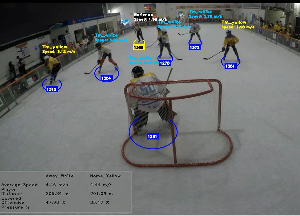
The ability to track teams and players opens up exciting possibilities for measuring performance, such as generating heatmaps, analyzing speed and distance covered, tracking movements like zone entries or exits, and diving into detailed player metrics. In order we can have a taste of it, we’ll add three performance metrics: average speed per player, skating distance covered by each team, and offensive pressure (measured as the percentage of distance covered by each team spent in its opponent’s zone). I’ll leave more detailed statistics up to you!
We begin adapting the coordinates of the ice rink from pixel-based measurements to approximate meters. This adjustment allows us to read our data in meters rather than pixels. The real-world dimensions of the ice rink seen in the video are approximately 15mx30m (15 meters in width and 30 meters in height). To facilitate this conversion, we introduce a method to convert pixel coordinates to meters. By defining the rink’s actual dimensions and using the pixel coordinates of its corners (from left to right and top to bottom), we obtain conversion factors. These factors will support our process of estimating distances in meters and speeds in meters per second. (Another interesting technique you can explore and apply is Perspective Transformation)
#*********************Loads models and rink coordinates*****************#
class_names = ['Referee', 'Tm_white', 'Tm_yellow']
class HockeyAnalyzer:
def __init__(self, model_path, classifier_path):
*
*
*
*
*
*
self.pixel_to_meter_conversion() #<------ Add this utility method
#***********Pixel-based measurements to meters***************************#
def pixel_to_meter_conversion(self):
#Rink real dimensions in meters
rink_width_m = 15
rink_height_m = 30
#Pixel coordinates for rink dimensions
left_pixel, right_pixel = self.rink_coordinates[0][0], self.rink_coordinates[1][0]
top_pixel, bottom_pixel = self.rink_coordinates[2][1], self.rink_coordinates[0][1]
#Conversion factors
self.pixels_per_meter_x = (right_pixel - left_pixel) / rink_width_m
self.pixels_per_meter_y = (bottom_pixel - top_pixel) / rink_height_m
def convert_pixels_to_meters(self, distance_pixels):
#Convert pixels to meters
return distance_pixels / self.pixels_per_meter_x, distance_pixels / self.pixels_per_meter_y
We are now ready to add speed to each player measured in meters per second. To do this, we’ll need to make three modifications. First, initiate an empty dictionary named previous_positions in the HockeyAnalyzer class to help us compare the current and previous positions of players. Similarly, we’ll create a team_stats structure to store stats from each team for further visualization.
Next, we will add a speed method to estimate players’ speed in pixels per second, and then use the conversion factor (explained earlier) to transform it into meters per second. Finally, from the analyze_video method, we’ll call our new speed method and add the speed to each tracked object (players and referee). This is what the changes look like:
#*********************Loads models and rink coordinates*****************#
class_names = ['Referee', 'Tm_white', 'Tm_yellow']
class HockeyAnalyzer:
def __init__(self, model_path, classifier_path):
*
*
*
*
*
*
*
self.pixel_to_meter_conversion()
self.previous_positions = {} #<------ Add this.Initializes empty dictionary
self.team_stats = {
'Tm_white': {'distance': 0, 'speed': [], 'count': 0, 'offensive_pressure': 0},
'Tm_yellow': {'distance': 0, 'speed': [], 'count': 0, 'offensive_pressure': 0}
} #<------ Add this.Initializes empty dictionary
#**************** Speed: meters per second********************************#
def calculate_speed(self, track_id, x_center, y_center, fps):
current_position = (x_center, y_center)
if track_id in self.previous_positions:
prev_position = self.previous_positions[track_id]
distance_pixels = np.linalg.norm(np.array(current_position) - np.array(prev_position))
distance_meters_x, distance_meters_y = self.convert_pixels_to_meters(distance_pixels)
speed_meters_per_second = (distance_meters_x**2 + distance_meters_y**2)**0.5 * fps
else:
speed_meters_per_second = 0
self.previous_positions[track_id] = current_position
return speed_meters_per_second
#******************* Loads Tracked Data (pickle file )**********************************#
def analyze_video(self, video_path, output_path, tracks_path):
with open(tracks_path, 'rb') as f:
tracks = pickle.load(f)
*
*
*
*
*
*
*
*
# Draw Team label
cv2.putText(
frame,
team,
(int(x1), int(y1) + text_offset),
cv2.FONT_HERSHEY_PLAIN,
font_scale,
text_color,
thickness=2
)
#**************Add these lines of code --->:
speed = self.calculate_speed(track_id, x_center, y_center, fps)
# Speed label
speed_font_scale = 0.8
speed_y_position = int(y1) + 20
if speed_y_position > int(y1) - 5:
speed_y_position = int(y1) - 5
cv2.putText(
frame,
f"Speed: {speed:.2f} m/s",
(int(x1), speed_y_position),
cv2.FONT_HERSHEY_PLAIN,
speed_font_scale,
text_color,
thickness=2
)
# Write output video
out.write(frame)
frame_num += 1
cap.release()
out.release()
If you have troubles adding this new lines of code, you can always visit the project’s GitHub repository, where you can find the complete integrated code. Your video output at this point should look like this (notice that the speed has been added to the label of each player):
Sample Clip 07: Tracking Players and Speed
Finally, let’s add a stats board where we can track the average speed per player for each team, along with other metrics such as distance covered and offensive pressure in the opponent’s zone.
We’ve already defined the offensive zones and integrated them into our code. Now, we need to track how often each player enters their opponent’s zone. To achieve this, we’ll implement a method using the ray casting algorithm. This algorithm checks if a player’s position is inside the white or yellow team’s offensive zone. It works by drawing an imaginary line from the player to the target zone. If the line crosses one border, the player is inside, if it crosses more (in our case, two out of four borders), the player is outside. The code then scans the entire video to determine each tracked object’s zone status.
#************ Locate player's position in Target Zone***********************#
def is_inside_zone(self, position, zone):
x, y = position
n = len(zone)
inside = False
p1x, p1y = zone[0]
for i in range(n + 1):
p2x, p2y = zone[i % n]
if y > min(p1y, p2y):
if y <= max(p1y, p2y):
if x <= max(p1x, p2x):
if p1y != p2y:
xinters = (y - p1y) * (p2x - p1x) / (p2y - p1y) + p1x
if p1x == p2x or x <= xinters:
inside = not inside
p1x, p1y = p2x, p2y
return inside
Now we’ll handle the performance metrics by adding a method that displays average player speed, total distance covered, and offensive pressure (percentage of time spent in the opponent’s zone) on a table format for each team. Using OpenCV, we’ll format these metrics into a table overlaid on the video and we’ll incorporate a dynamic update mechanism to maintain real-time statistics during gameplay.
#*******************************Performance metrics*********************************************#
def draw_stats(self, frame):
avg_speed_white = np.mean(self.team_stats['Tm_white']['speed']) if self.team_stats['Tm_white']['count'] > 0 else 0
avg_speed_yellow = np.mean(self.team_stats['Tm_yellow']['speed']) if self.team_stats['Tm_yellow']['count'] > 0 else 0
distance_white = self.team_stats['Tm_white']['distance']
distance_yellow = self.team_stats['Tm_yellow']['distance']
offensive_pressure_white = self.team_stats['Tm_white'].get('offensive_pressure', 0)
offensive_pressure_yellow = self.team_stats['Tm_yellow'].get('offensive_pressure', 0)
Pressure_ratio_W = offensive_pressure_white/distance_white *100 if self.team_stats['Tm_white']['distance'] > 0 else 0
Pressure_ratio_Y = offensive_pressure_yellow/distance_yellow *100 if self.team_stats['Tm_yellow']['distance'] > 0 else 0
table = [
["", "Away_White", "Home_Yellow"],
["Average Speed\nPlayer", f"{avg_speed_white:.2f} m/s", f"{avg_speed_yellow:.2f} m/s"],
["Distance\nCovered", f"{distance_white:.2f} m", f"{distance_yellow:.2f} m"],
["Offensive\nPressure %", f"{Pressure_ratio_W:.2f} %", f"{Pressure_ratio_Y:.2f} %"],
]
text_color = (0, 0, 0)
start_x, start_y = 10, 590
row_height = 30 # Manage Height between rows
column_width = 150 # Manage Width between rows
font_scale = 1
def put_multiline_text(frame, text, position, font, font_scale, color, thickness, line_type, line_spacing=1.0):
y0, dy = position[1], int(font_scale * 20 * line_spacing) # Adjust line spacing here
for i, line in enumerate(text.split('\n')):
y = y0 + i * dy
cv2.putText(frame, line, (position[0], y), font, font_scale, color, thickness, line_type)
for i, row in enumerate(table):
for j, text in enumerate(row):
if i in [1,2, 3]:
put_multiline_text(
frame,
text,
(start_x + j * column_width, start_y + i * row_height),
cv2.FONT_HERSHEY_PLAIN,
font_scale,
text_color,
1,
cv2.LINE_AA,
line_spacing= 0.8
)
else:
cv2.putText(
frame,
text,
(start_x + j * column_width, start_y + i * row_height),
cv2.FONT_HERSHEY_PLAIN,
font_scale,
text_color,
1,
cv2.LINE_AA,
)
#****************** Track and update game stats****************************************#
def update_team_stats(self, team, speed, distance, position):
if team in self.team_stats:
self.team_stats[team]['speed'].append(speed)
self.team_stats[team]['distance'] += distance
self.team_stats[team]['count'] += 1
if team == 'Tm_white':
if self.is_inside_zone(position, self.zone_white):
self.team_stats[team]['offensive_pressure'] += distance
elif team == 'Tm_yellow':
if self.is_inside_zone(position, self.zone_yellow):
self.team_stats[team]['offensive_pressure'] += distance
In order the stats display in the video we’ll have to call the method in the analyze_video method, so be sure to add this extra lines of code after the speed label is defined and just before the output video is processed:
*
*
*
*
*
*
*
#Speed label
speed_font_scale = 0.8
speed_y_position = int(y1) + 20
if speed_y_position > int(y1) - 5:
speed_y_position = int(y1) - 5
cv2.putText(
frame,
f"Speed: {speed:.2f} m/s",
(int(x1), speed_y_position),
cv2.FONT_HERSHEY_PLAIN,
speed_font_scale,
text_color,
thickness=2
)
#**************Add these lines of code--->:
distance = speed / fps
position = (x_center, y_center)
self.update_team_stats(team, speed, distance, position)
# Write output video
out.write(frame)
frame_num += 1
The distance in meters covered by each player is calculated by dividing their speed (measured in meters per second) by the frame rate (frames per second). This calculation allows us to estimate how far each player moves between each frame change in the video. If everything works well, your final video output should look like this:
Sample Clip 08: Final Output
Considerations and Future Work
This model is a basic setup of what can be achieved using computer vision to track players in an ice hockey game (or any team sport). However, there’s a lot of fine-tuning that can be done to improve it and add new capabilities. Here are a few ideas that I’m working on for a next 2.0 version that you might also consider:
The challenge of following the puck: Depending on which direction your camera is facing and the resolution, tracking the puck is challenging considering its size compared to a soccer or basketball ball. But if you achieve this, interesting possibilities open up to track performance, such as possession time metrics, goal opportunities, or shots data. This also applies also to individual performances; in ice hockey, players change significantly more often than in other team sports, so tracking each player’s performance during one period presents a challenge.
Compute resources, Oh why compute! I ran all the code on a CPU arrangement but faced issues (sometimes resulting in blue screens 😥) due to running out of memory during the design process (consider using a CUDA setup). Our sample video is about 40 seconds long and initially 5 MB in size, but after running the model, the output increases to up to 34 MB. Imagine the size for a full 20-minute game period. So, you should consider compute resources and storage when scaling up.
Don’t underestimate MLOps: To deploy and scale rapidly, we need Machine Learning pipelines that are efficient, support frequent execution, and are reliable. This involves considering a Continuous Integration-Deployment-Training approach. Our use case has been built for a specific scenario, but what if conditions change, such as the camera direction or jersey colors? To scale up, we must adopt a CI/CD/CT mindset.
I hope you found this computer vision project interesting, you can access the complete code in this GitHub repository. And if you want to support the development of inline and ice hockey in the region, follow the APHL (we are always in need of used equipment you’d like to donate for young players and working on building our first official hockey rink), and worldwide, follow and support the Friendship League.
Did I miss anything? Your suggestions are always welcome. Let’s keep the conversation going!
Spicing up Ice Hockey with AI: Player Tracking with Computer Vision was originally published in Towards Data Science on Medium, where people are continuing the conversation by highlighting and responding to this story.