Comparing model-free and model-based RL methods on a dynamic grid world

Photo by Saffu on Unsplash
Recently, Reinforcement Learning (RL) algorithms have received a lot of traction by solving research problems such as protein folding, reaching a superhuman level in drone racing, or even integrating human feedback in your favorite chatbots.
Indeed, RL provides useful solutions to a variety of sequential decision-making problems. Temporal-Difference Learning (TD learning) methods are a popular subset of RL algorithms. TD learning methods combine key aspects of Monte Carlo and Dynamic Programming methods to accelerate learning without requiring a perfect model of the environment dynamics.
In this article, we’ll compare different kinds of TD algorithms in a custom Grid World. The design of the experiment will outline the importance of continuous exploration as well as the individual characteristics of the tested algorithms: Q-learning, Dyna-Q, and Dyna-Q+.
The outline of this post contains:
The full code allowing the reproduction of the results and the plots is available here: https://github.com/RPegoud/Temporal-Difference-learning
The Environment
The environment we’ll use in this experiment is a grid world with the following features:

Description of the different components of the Grid World (Made by the author)
This experiment aims to compare the behavior of Q-learning, Dyna-Q, and Dyna-Q+ agents in a changing environment. Indeed, after 100 episodes, the optimal policy is bound to change and the optimal number of steps during a successful episode will decrease from 17 to 12.

Representation of the grid world, optimal paths depend on the current episode (made by the author)
Introduction to Temporal-Difference Learning:
Temporal-Difference Learning is a combination of Monte Carlo (MC) and Dynamic Programming (DP) methods:
One particularity of TD methods is that they update their value estimate every time step, as opposed to MC methods that wait until the end of an episode.
Indeed, both methods have different update targets. MC methods aim to update the return Gt, which is only available at the end of an episode. Instead, TD methods target:
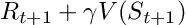
Update target for TD methods
Where V is an estimate of the true value function Vπ.
Therefore, TD methods combine the sampling of MC (by using an estimate of the true value) and the bootstrapping of DP (by updating V based on estimates relying on further estimates).
The simplest version of temporal-difference learning is called TD(0) or one-step TD, a practical implementation of TD(0) would look like this:
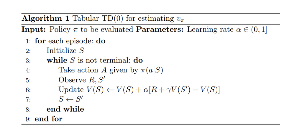
Pseudo-code for the TD(0) algorithm, reproduced from Reinforcement Learning, an introduction [4]
When transitioning from a state S to a new state S’, the TD(0) algorithm will compute a backed-up value and update V(S) accordingly. This backed-up value is called TD error, the difference between the optimal value function V_star and our current estimate V(S):

The TD error
In conclusion, TD methods present several advantages:
The following sections explore several TD algorithms’ main characteristics and performance son the grid world.
The same parameters were used for all models, for the sake of simplicity:
The performances of each algorithm are first presented for a single run of 400 episodes (sections: Q-learning, Dyna-Q, and Dyna-Q+) and then averaged over 100 runs of 250 episodes in the “summary and algorithms comparison” section.
Q-learning
The first algorithm we implement here is the famous Q-learning (Watkins, 1989):

Q-learning is called an off-policy algorithm as its goal is to approximate the optimal value function directly, instead of the value function of π, the policy followed by the agent.
In practice, Q-learning still relies on a policy, often referred to as the ‘behavior policy’ to select which state-action pairs are visited and updated. However, Q-learning is off-policy becauseit updates its Q-values based on the best estimate of future rewards, regardless of whether the selected actions follow the current policy π.
Compared to the previous TD learning pseudo-code, there are three main differences:
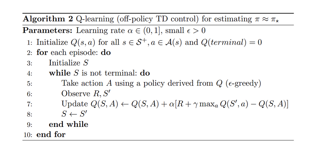
Pseudo-code for the Q-learning algorithm, reproduced from Reinforcement Learning, an introduction [4]
Now that we have our first algorithm reading for testing, we can start the training phase. Our agent will navigate the Grid World using its ε-greedy policy, with respect to the Q values. This policy selects the action with the highest Q-value with a probability of (1 - ε) and chooses a random action with a probability of ε. After each action, the agent will update its Q-value estimates.
We can visualize the evolution of the estimated maximum action-value Q(S, a) of each cell of the Grid World using a heatmap. Here the agent plays 400 episodes. As there is only one update per episode, the evolution of the Q values is quite slow and a large part of the states remain unmapped:

Heatmap representation of the learned Q values of each state, during training (made by the author)
Upon completion of the 400 episodes, an analysis of the total visits to each cell provides us with a decent estimate of the agent’s average route. As depicted on the right-hand plot below, the agent seems to have converged to a sub-optimal route, avoiding cell (4,4) and consistently following the lower wall.
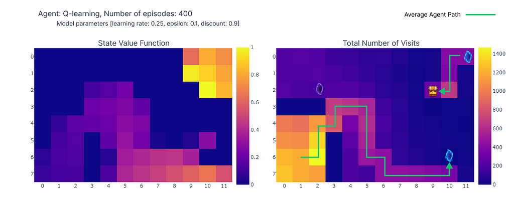
(left) Estimation of the maximal action value for each state, (right) Number of visits per state (made by the author)
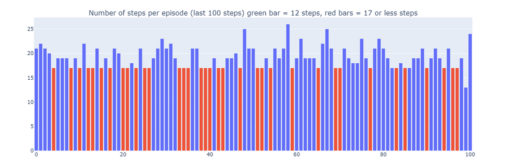
As a result of this sub-optimal strategy, the agent reaches a minimum of 21 steps per episode, following the path outlined in the “number of total visits” plot. Variations in step counts can be attributed to the ε-greedy policy, which introduces a 10% probability of random actions. Given this policy, following the lower wall is a decent strategy to limit potential disruptions caused by random actions.
Number of steps for the last 100 episodes of training (300–400) (made by the author)
In conclusion, the Q-learning agent converged to a sub-optimal strategy as mentioned previously. Moreover, a portion of the environment remains unexplored by the Q-function, which prevents the agent from finding the new optimal path when the purple portal appears after the 100th episode.
These performance limitations can be attributed to the relatively low number of training steps (400), limiting the possibilities of interaction with the environment and the exploration induced by the ε-greedy policy.
Planning, an essential component of model-based reinforcement learning methods is particularly useful to improve sample efficiency and estimation of action values. Dyna-Q and Dyna-Q+ are good examples of TD algorithms incorporating planning steps.
Dyna-Q
The Dyna-Q algorithm (Dynamic Q-learning) is a combination of model-based RL and TD learning.
Model-based RL algorithms rely on a model of the environment to incorporate planning as their primary way of updating value estimates. In contrast, model-free algorithms rely on direct learning.
In the scope of this article, the model can be seen as an approximation of the transition dynamics p(s’, r|s, a). Here, p returns a single next-state and reward pair given the current state-action pair.
In environments where p is stochastic, we distinguish distribution models and sample models, the former returns a distribution of the next states and actions while the latter returns a single pair, sampled from the estimated distribution.
Models are especially useful to simulate episodes, and therefore train the agent by replacing real-world interactions with planning steps, i.e. interactions with the simulated environment.
Agents implementing the Dyna-Q algorithm are part of the class of planning agents, agents that combine direct reinforcement learning and model learning. They use direct interactions with the environment to update their value function (as in Q-learning) and also to learn a model of the environment. After each direct interaction, they can also perform planning steps to update their value function using simulated interactions.
A quick Chess example
Imagine playing a good game of chess. After playing each move, the reaction of your opponent allows you to assess the quality of your move. This is similar to receiving a positive or negative reward, which allows you to “update” your strategy. If your move leads to a blunder, you probably wouldn’t do it again, provided with the same configuration of the board. So far, this is comparable to direct reinforcement learning.
Now let’s add planning to the mix. Imagine that after each of your moves, while the opponent is thinking, you mentally go back over each of your previous moves to reassess their quality. You might find weaknesses that you neglected at first sight or find out that specific moves were better than you thought. These thoughts may also allow you to update your strategy. This is exactly what planning is about, updating the value function without interacting with the real environment but rather a model of said environment.
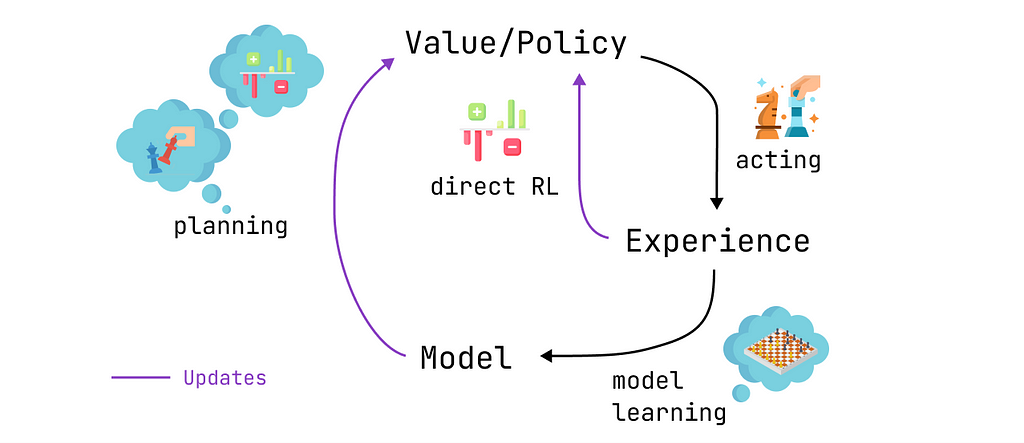
Planning, acting, model learning, and direct RL: the schedule of a planning agent (made by the author)
Dyna-Q therefore contains some additional steps compared to Q-learning:
After each direct update of the Q values, the model stores the state-action pair and the reward and next-state that were observed. This step is called model training.
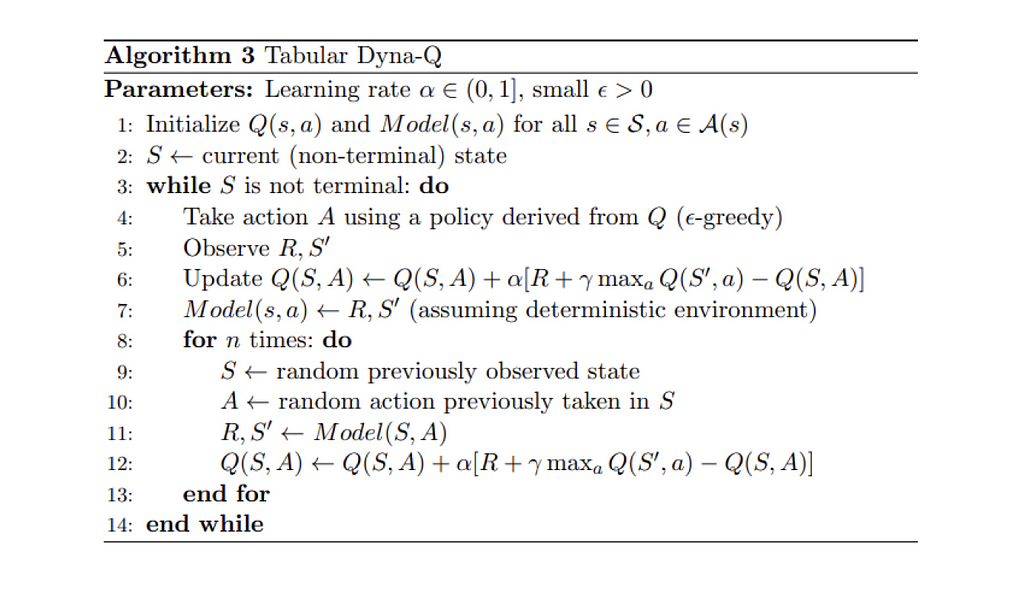
Pseudo-code for the Dyna-Q algorithm, reproduced from Reinforcement Learning, an introduction [4]
We now replicate the learning process with the Dyna-Q algorithm using n=100. This means that after each direct interaction with the environment, we use the model to perform 100 planning steps (i.e. updates).
The following heatmap shows the fast convergence of the Dyna-Q model. In fact, it only takes the algorithm around 10 episodes to find an optimal path. This is due to the fact that every step leads to 101 updates of the Q values (instead of 1 for Q-learning).

Heatmap representation of the learned Q values of each state during training (made by the author)
Another benefit of planning steps is a better estimation of action values across the grid. As the indirect updates target random transitions stored inside the model, states that are far away from the goal also get updated.
In contrast, the action values slowly propagate from the goal in Q-learning, leading to an incomplete mapping of the grid.
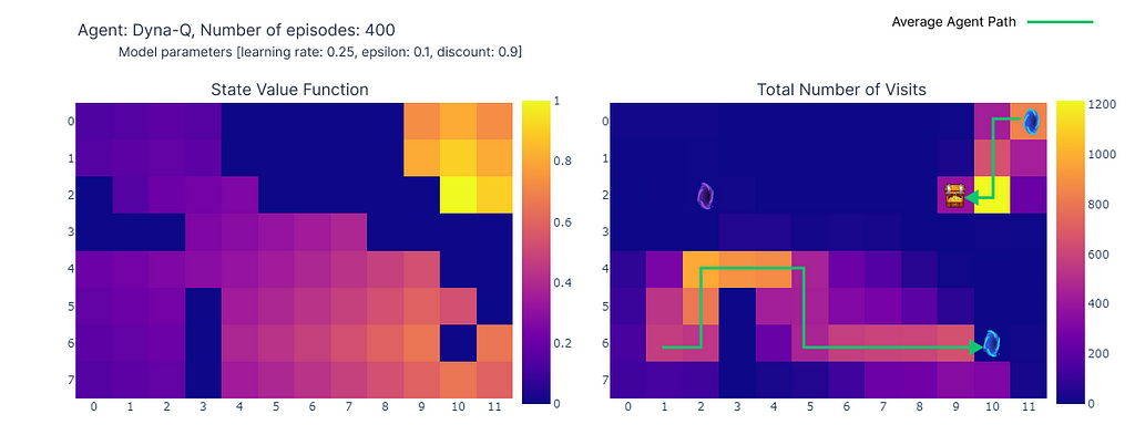
(left) Estimation of the maximal action value for each state, (right) Number of visits per state (made by the author)
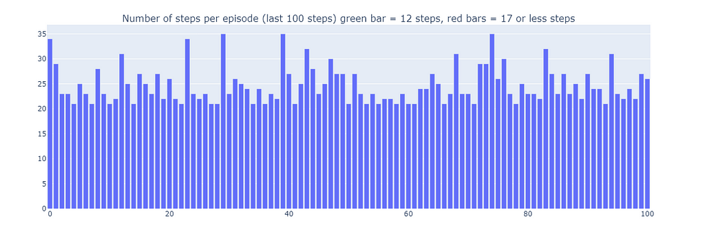
Using Dyna-Q, we find an optimal path allowing the resolution of the grid world in 17 steps, as depicted on the plot below by red bars. Optimal performances are attained regularly, despite the occasional interference of ε-greedy actions for the sake of exploration.
Finally, while Dyna-Q may appear more convincing than Q-learning due to its incorporation of planning, it’s essential to remember that planning introduces a tradeoff between computational costs and real-world exploration.
Number of steps for the last 100 episodes of training (300–400) (made by the author)
Dyna-Q+
Up to now, neither of the tested algorithms managed to find the optimal path appearing after step 100 (the purple portal). Indeed, both algorithms rapidly converged to an optimal solution that remained fixed until the end of the training phase. This highlights the need for continuous exploration throughout training.
Dyna-Q+ is largely similar to Dyna-Q but adds a small twist to the algorithm. Indeed, Dyna-Q+ constantly tracks the number of time steps elapsed since each state-action pair was tried in real interaction with the environment.
In particular, consider a transition yielding a reward r that has not been tried in τ time steps. Dyna-Q+ would perform planning as if the reward for this transition was r + κ √τ, with κ sufficiently small (0.001 in the experiment).
This change in reward design encourages the agent to continually explore the environment. It assumes that the longer a state-action pair hasn’t been tried, the greater the chances that the dynamics of this pair have changed or that the model is incorrect.

Pseudo-code for the Dyna-Q+ algorithm, reproduced from Reinforcement Learning, an introduction [4]
As depicted by the following heatmap, Dyna-Q+ is much more active with its updates compared to the previous algorithms. Before episode 100, the agent explores the whole grid and finds the blue portal and the first optimal route.
The action values for the rest of the grid decrease before slowly increasing again, as states-action pairs in the top left corner are not explored for some time.
As soon as the purple portal appears in episode 100, the agent finds the new shortcut and the value for the whole area rises. Until the completion of the 400 episodes, the agent will continuously update the action value of each state-action pair while maintaining occasional exploration of the grid.

Heatmap representation of the learned Q values of each state, during training (made by the author)
Thanks to the bonus added to model rewards, we finally obtain a complete mapping of the Q function (each state or cell has an action value).
Combined with continuous exploration, the agent manages to find the new best route (i.e. optimal policy) as it appears, while retaining the previous solution.

(left) Estimation of the maximal action value for each state, (right) Number of visits per state (made by the author)
However, the exploration-exploitation trade-off in Dyna-Q+ indeed comes with a cost. When state-action pairs haven’t been visited for a sufficient duration, the exploration bonus encourages the agent to revisit those states, which can temporarily decrease its immediate performance. This exploration behavior prioritizes updating the model to improve long-term decision-making.
This explains why some episodes played by Dyna-Q+ can be up to 70 steps long, compared to at most 35 and 25 steps for Q-learning and Dyna-Q, respectively. The longer episodes in Dyna-Q+ reflect the agent’s willingness to invest extra steps in exploration to gather more information about the environment and refine its model, even if it results in short-term performance reductions.
In contrast, Dyna-Q+ regularly achieves optimal performance (depicted by green bars on the plot below) that previous algorithms did not attain.
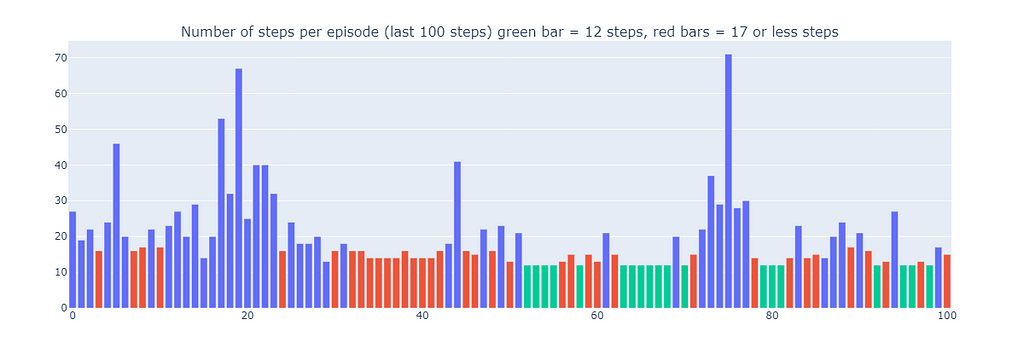
Number of steps for the last 100 episodes of training (300–400) (made by the author)
Summary and Algorithms Comparison
In order to compare the key differences between the algorithms, we use two metrics (keep in mind that the results depend on the input parameters, which were identical among all models for simplicity):
Analyzing the number of steps per episode (see plot below), reveals several aspects of model-based and model-free methods:
Comparison of the number of steps per episode averaged over 100 runs (made by the author)
We now introduce the average cumulative reward (ACR), which represents the percentage of episodes where the agent reaches the goal (as the reward is 1 for reaching the goal and 0 for triggering a trap), the ACR is then simply by:

With N the number of episodes (250) and K the number of independent runs (100) and Rn,k the cumulative reward for episode n in run k.
Here’s a breakdown of the performance of all algorithms:

Comparison of the cumulative reward per episode averaged over 100 runs (made by the author)
Conclusion
In this article, we presented the fundamental principles of Temporal Difference learning and applied Q-learning, Dyna-Q, and Dyna-Q+ to a custom grid world. The design of this grid world helps emphasize the importance of continual exploration as a way to discover and exploit new optimal policies in changing environments. The difference in performances (evaluated using the number of steps per episode and the cumulative reward) illustrate the strengths and weaknesses of these algorithms.
In summary, model-based methods (Dyna-Q, Dyna-Q+) benefit from increased sample efficiency compared to model-based methods (Q-learning), at the cost of computation efficiency. However, in stochastic or more complex environments, inaccuracies in the model could hinder performances and lead to sub-optimal policies.
References:
[1] Demis Hassabis, AlphaFold reveals the structure of the protein universe (2022), DeepMind
[2] Elia Kaufmann, Leonard Bauersfeld, Antonio Loquercio, Matthias Müller, Vladlen Koltun &Davide Scaramuzza, Champion-level drone racing using deep reinforcement learning (2023), Nature
[3] Nathan Lambert, LouisCastricato, Leandro von Werra, Alex Havrilla, Illustrating Reinforcement Learning from Human Feedback (RLHF), HuggingFace
[4] Sutton, R. S., & Barto, A. G. . Reinforcement Learning: An Introduction (2018), Cambridge (Mass.): The MIT Press.
[5] Christopher J. C. H. Watkins & Peter Dayan, Q-learning (1992), Machine Learning, Springer Link

Temporal-Difference Learning and the importance of exploration: An illustrated guide was originally published in Towards Data Science on Medium, where people are continuing the conversation by highlighting and responding to this story.
Photo by Saffu on Unsplash
Recently, Reinforcement Learning (RL) algorithms have received a lot of traction by solving research problems such as protein folding, reaching a superhuman level in drone racing, or even integrating human feedback in your favorite chatbots.
Indeed, RL provides useful solutions to a variety of sequential decision-making problems. Temporal-Difference Learning (TD learning) methods are a popular subset of RL algorithms. TD learning methods combine key aspects of Monte Carlo and Dynamic Programming methods to accelerate learning without requiring a perfect model of the environment dynamics.
In this article, we’ll compare different kinds of TD algorithms in a custom Grid World. The design of the experiment will outline the importance of continuous exploration as well as the individual characteristics of the tested algorithms: Q-learning, Dyna-Q, and Dyna-Q+.
The outline of this post contains:
- Description of the environment
- Temporal-Difference (TD) Learning
- Model-free TD methods (Q-learning) and model-based TD methods (Dyna-Q and Dyna-Q+)
- Parameters
- Performance comparisons
- Conclusion
The full code allowing the reproduction of the results and the plots is available here: https://github.com/RPegoud/Temporal-Difference-learning
The Environment
The environment we’ll use in this experiment is a grid world with the following features:
- The grid is 12 by 8 cells.
- The agent starts in the bottom left corner of the grid, the objective is to reach the treasure located in the top right corner (a terminal state with reward 1).
- The blue portals are connected, going through the portal located on the cell (10, 6) leads to the cell (11, 0). The agent cannot take the portal again after its first transition.
- The purple portal only appears after 100 episodes but enables the agent to reach the treasure faster. This encourages continually exploring the environment.
- The red portals are traps (terminal states with reward 0) and end the episode.
- Bumping into a wall causes the agent to remain in the same state.
Description of the different components of the Grid World (Made by the author)
This experiment aims to compare the behavior of Q-learning, Dyna-Q, and Dyna-Q+ agents in a changing environment. Indeed, after 100 episodes, the optimal policy is bound to change and the optimal number of steps during a successful episode will decrease from 17 to 12.
Representation of the grid world, optimal paths depend on the current episode (made by the author)
Introduction to Temporal-Difference Learning:
Temporal-Difference Learning is a combination of Monte Carlo (MC) and Dynamic Programming (DP) methods:
- Like MC methods, TD methods can learn from experience without requiring a model of the environment’s dynamics.
- Like DP methods, TD methods update estimates after every step based on other learned estimates without waiting for the outcome (this is called bootstrapping).
One particularity of TD methods is that they update their value estimate every time step, as opposed to MC methods that wait until the end of an episode.
Indeed, both methods have different update targets. MC methods aim to update the return Gt, which is only available at the end of an episode. Instead, TD methods target:
Update target for TD methods
Where V is an estimate of the true value function Vπ.
Therefore, TD methods combine the sampling of MC (by using an estimate of the true value) and the bootstrapping of DP (by updating V based on estimates relying on further estimates).
The simplest version of temporal-difference learning is called TD(0) or one-step TD, a practical implementation of TD(0) would look like this:
Pseudo-code for the TD(0) algorithm, reproduced from Reinforcement Learning, an introduction [4]
When transitioning from a state S to a new state S’, the TD(0) algorithm will compute a backed-up value and update V(S) accordingly. This backed-up value is called TD error, the difference between the optimal value function V_star and our current estimate V(S):
The TD error
In conclusion, TD methods present several advantages:
- They do not require a perfect model of the environment’s dynamics p
- They are implemented in an online fashion, updating the target after each time step
- TD(0) is guaranteed to converge for any fixed policy π if α (the learning rate or step size) follows stochastic approximation conditions (for more detail see page 55 ”Tracking a Nonstationary Problem” of [4])
The following sections explore several TD algorithms’ main characteristics and performance son the grid world.
The same parameters were used for all models, for the sake of simplicity:
- Epsilon (ε) = 0.1: probability of selecting a random action in ε-greedy policies
- Gamma (γ)= 0.9: discount factor applied to future rewards or value estimates
- Aplha (α) = 0.25: learning rate restricting the Q value updates
- Planning steps = 100: for Dyna-Q and Dyna-Q+, the number of planning steps executed for each direct interaction
- Kappa (κ)= 0.001: for Dyna-Q+, the weight of bonus rewards applied during planning steps
The performances of each algorithm are first presented for a single run of 400 episodes (sections: Q-learning, Dyna-Q, and Dyna-Q+) and then averaged over 100 runs of 250 episodes in the “summary and algorithms comparison” section.
Q-learning
The first algorithm we implement here is the famous Q-learning (Watkins, 1989):
Q-learning is called an off-policy algorithm as its goal is to approximate the optimal value function directly, instead of the value function of π, the policy followed by the agent.
In practice, Q-learning still relies on a policy, often referred to as the ‘behavior policy’ to select which state-action pairs are visited and updated. However, Q-learning is off-policy becauseit updates its Q-values based on the best estimate of future rewards, regardless of whether the selected actions follow the current policy π.
Compared to the previous TD learning pseudo-code, there are three main differences:
- We need to initialize the Q function for all states and actions and Q(terminal) should be 0
- The actions are chosen from a policy based on the Q values (for instance the ϵ-greedy policy with respect to the Q values)
- The update targets the action value function Q rather than the state value function V
Pseudo-code for the Q-learning algorithm, reproduced from Reinforcement Learning, an introduction [4]
Now that we have our first algorithm reading for testing, we can start the training phase. Our agent will navigate the Grid World using its ε-greedy policy, with respect to the Q values. This policy selects the action with the highest Q-value with a probability of (1 - ε) and chooses a random action with a probability of ε. After each action, the agent will update its Q-value estimates.
We can visualize the evolution of the estimated maximum action-value Q(S, a) of each cell of the Grid World using a heatmap. Here the agent plays 400 episodes. As there is only one update per episode, the evolution of the Q values is quite slow and a large part of the states remain unmapped:
Heatmap representation of the learned Q values of each state, during training (made by the author)
Upon completion of the 400 episodes, an analysis of the total visits to each cell provides us with a decent estimate of the agent’s average route. As depicted on the right-hand plot below, the agent seems to have converged to a sub-optimal route, avoiding cell (4,4) and consistently following the lower wall.
(left) Estimation of the maximal action value for each state, (right) Number of visits per state (made by the author)
As a result of this sub-optimal strategy, the agent reaches a minimum of 21 steps per episode, following the path outlined in the “number of total visits” plot. Variations in step counts can be attributed to the ε-greedy policy, which introduces a 10% probability of random actions. Given this policy, following the lower wall is a decent strategy to limit potential disruptions caused by random actions.
Number of steps for the last 100 episodes of training (300–400) (made by the author)
In conclusion, the Q-learning agent converged to a sub-optimal strategy as mentioned previously. Moreover, a portion of the environment remains unexplored by the Q-function, which prevents the agent from finding the new optimal path when the purple portal appears after the 100th episode.
These performance limitations can be attributed to the relatively low number of training steps (400), limiting the possibilities of interaction with the environment and the exploration induced by the ε-greedy policy.
Planning, an essential component of model-based reinforcement learning methods is particularly useful to improve sample efficiency and estimation of action values. Dyna-Q and Dyna-Q+ are good examples of TD algorithms incorporating planning steps.
Dyna-Q
The Dyna-Q algorithm (Dynamic Q-learning) is a combination of model-based RL and TD learning.
Model-based RL algorithms rely on a model of the environment to incorporate planning as their primary way of updating value estimates. In contrast, model-free algorithms rely on direct learning.
”A model of the environment is anything that an agent can use to predict how the environment will respond to its actions” — Reinforcement Learning: an introduction.
In the scope of this article, the model can be seen as an approximation of the transition dynamics p(s’, r|s, a). Here, p returns a single next-state and reward pair given the current state-action pair.
In environments where p is stochastic, we distinguish distribution models and sample models, the former returns a distribution of the next states and actions while the latter returns a single pair, sampled from the estimated distribution.
Models are especially useful to simulate episodes, and therefore train the agent by replacing real-world interactions with planning steps, i.e. interactions with the simulated environment.
Agents implementing the Dyna-Q algorithm are part of the class of planning agents, agents that combine direct reinforcement learning and model learning. They use direct interactions with the environment to update their value function (as in Q-learning) and also to learn a model of the environment. After each direct interaction, they can also perform planning steps to update their value function using simulated interactions.
A quick Chess example
Imagine playing a good game of chess. After playing each move, the reaction of your opponent allows you to assess the quality of your move. This is similar to receiving a positive or negative reward, which allows you to “update” your strategy. If your move leads to a blunder, you probably wouldn’t do it again, provided with the same configuration of the board. So far, this is comparable to direct reinforcement learning.
Now let’s add planning to the mix. Imagine that after each of your moves, while the opponent is thinking, you mentally go back over each of your previous moves to reassess their quality. You might find weaknesses that you neglected at first sight or find out that specific moves were better than you thought. These thoughts may also allow you to update your strategy. This is exactly what planning is about, updating the value function without interacting with the real environment but rather a model of said environment.
Planning, acting, model learning, and direct RL: the schedule of a planning agent (made by the author)
Dyna-Q therefore contains some additional steps compared to Q-learning:
After each direct update of the Q values, the model stores the state-action pair and the reward and next-state that were observed. This step is called model training.
- After model training, Dyna-Q performs n planning steps:
- A random state-action pair is selected from the model buffer (i.e. this state-action pair was observed during direct interactions)
- The model generates the simulated reward and next-state
- The value function is updated using the simulated observations (s, a, r, s’)
Pseudo-code for the Dyna-Q algorithm, reproduced from Reinforcement Learning, an introduction [4]
We now replicate the learning process with the Dyna-Q algorithm using n=100. This means that after each direct interaction with the environment, we use the model to perform 100 planning steps (i.e. updates).
The following heatmap shows the fast convergence of the Dyna-Q model. In fact, it only takes the algorithm around 10 episodes to find an optimal path. This is due to the fact that every step leads to 101 updates of the Q values (instead of 1 for Q-learning).
Heatmap representation of the learned Q values of each state during training (made by the author)
Another benefit of planning steps is a better estimation of action values across the grid. As the indirect updates target random transitions stored inside the model, states that are far away from the goal also get updated.
In contrast, the action values slowly propagate from the goal in Q-learning, leading to an incomplete mapping of the grid.
(left) Estimation of the maximal action value for each state, (right) Number of visits per state (made by the author)
Using Dyna-Q, we find an optimal path allowing the resolution of the grid world in 17 steps, as depicted on the plot below by red bars. Optimal performances are attained regularly, despite the occasional interference of ε-greedy actions for the sake of exploration.
Finally, while Dyna-Q may appear more convincing than Q-learning due to its incorporation of planning, it’s essential to remember that planning introduces a tradeoff between computational costs and real-world exploration.
Number of steps for the last 100 episodes of training (300–400) (made by the author)
Dyna-Q+
Up to now, neither of the tested algorithms managed to find the optimal path appearing after step 100 (the purple portal). Indeed, both algorithms rapidly converged to an optimal solution that remained fixed until the end of the training phase. This highlights the need for continuous exploration throughout training.
Dyna-Q+ is largely similar to Dyna-Q but adds a small twist to the algorithm. Indeed, Dyna-Q+ constantly tracks the number of time steps elapsed since each state-action pair was tried in real interaction with the environment.
In particular, consider a transition yielding a reward r that has not been tried in τ time steps. Dyna-Q+ would perform planning as if the reward for this transition was r + κ √τ, with κ sufficiently small (0.001 in the experiment).
This change in reward design encourages the agent to continually explore the environment. It assumes that the longer a state-action pair hasn’t been tried, the greater the chances that the dynamics of this pair have changed or that the model is incorrect.
Pseudo-code for the Dyna-Q+ algorithm, reproduced from Reinforcement Learning, an introduction [4]
As depicted by the following heatmap, Dyna-Q+ is much more active with its updates compared to the previous algorithms. Before episode 100, the agent explores the whole grid and finds the blue portal and the first optimal route.
The action values for the rest of the grid decrease before slowly increasing again, as states-action pairs in the top left corner are not explored for some time.
As soon as the purple portal appears in episode 100, the agent finds the new shortcut and the value for the whole area rises. Until the completion of the 400 episodes, the agent will continuously update the action value of each state-action pair while maintaining occasional exploration of the grid.
Heatmap representation of the learned Q values of each state, during training (made by the author)
Thanks to the bonus added to model rewards, we finally obtain a complete mapping of the Q function (each state or cell has an action value).
Combined with continuous exploration, the agent manages to find the new best route (i.e. optimal policy) as it appears, while retaining the previous solution.
(left) Estimation of the maximal action value for each state, (right) Number of visits per state (made by the author)
However, the exploration-exploitation trade-off in Dyna-Q+ indeed comes with a cost. When state-action pairs haven’t been visited for a sufficient duration, the exploration bonus encourages the agent to revisit those states, which can temporarily decrease its immediate performance. This exploration behavior prioritizes updating the model to improve long-term decision-making.
This explains why some episodes played by Dyna-Q+ can be up to 70 steps long, compared to at most 35 and 25 steps for Q-learning and Dyna-Q, respectively. The longer episodes in Dyna-Q+ reflect the agent’s willingness to invest extra steps in exploration to gather more information about the environment and refine its model, even if it results in short-term performance reductions.
In contrast, Dyna-Q+ regularly achieves optimal performance (depicted by green bars on the plot below) that previous algorithms did not attain.
Number of steps for the last 100 episodes of training (300–400) (made by the author)
Summary and Algorithms Comparison
In order to compare the key differences between the algorithms, we use two metrics (keep in mind that the results depend on the input parameters, which were identical among all models for simplicity):
- Number of steps per episode: this metric characterizes the rate of convergence of the algorithms towards an optimal solution. It also describes the behavior of the algorithm after convergence, particularly in terms of exploration.
- Average cumulative reward: the percentage of episodes leading to a positive reward
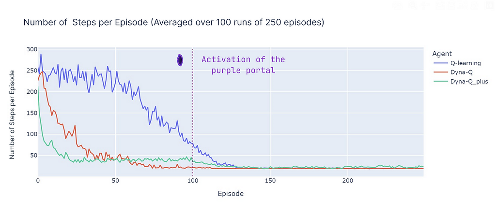
Analyzing the number of steps per episode (see plot below), reveals several aspects of model-based and model-free methods:
- Model-Based Efficiency: Model-based algorithms (Dyna-Q and Dyna-Q+) tend to be more sample-efficient in this particular Grid World (this property is also observed more generally in RL). This is because they can plan ahead using the learned model of the environment, which can lead to quicker convergence to near optimal or optimal solutions.
- Q-Learning Convergence: Q-learning, while eventually converging to a near optimal solution, requires more episodes (125) to do so. It’s important to highlight that Q-learning performs only 1 update per step, which contrasts with the multiple updates performed by Dyna-Q and Dyna-Q+.
- Multiple Updates: Dyna-Q and Dyna-Q+ execute 101 updates per step, which contributes to their faster convergence. However the tradeoff for this sample-efficiency is computational cost (see the runtime section in the table below).
- Complex Environments: In more complex or stochastic environments, the advantage of model-based methods might diminish. Models can introduce errors or inaccuracies, which can lead to suboptimal policies. Therefore, this comparison should be seen as an outline of the strengths and weaknesses of different approaches rather than a direct performance comparison.
Comparison of the number of steps per episode averaged over 100 runs (made by the author)
We now introduce the average cumulative reward (ACR), which represents the percentage of episodes where the agent reaches the goal (as the reward is 1 for reaching the goal and 0 for triggering a trap), the ACR is then simply by:
With N the number of episodes (250) and K the number of independent runs (100) and Rn,k the cumulative reward for episode n in run k.
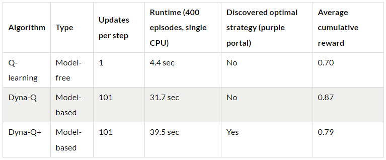
Here’s a breakdown of the performance of all algorithms:
- Dyna-Q converges rapidly and achieves the highest overall return, with an ACR of 87%. This means that it efficiently learns and reaches the goal in a significant portion of episodes.
- Q-learning also reaches a similar level of performance but requires more episodes to converge, explaining its slightly lower ACR, at 70%.
- Dyna-Q+ promptly finds a good policy, reaching a cumulative reward of 0.8 after only 15 episodes. However, the variability and exploration induced by the bonus reward reduces performance until step 100. After 100 steps, it starts to improve as it discovers the new optimal path. However, the short-term exploration compromises its performance, resulting in an ACR of 79%, which is lower than Dyna-Q but higher than Q-learning.
Comparison of the cumulative reward per episode averaged over 100 runs (made by the author)
Conclusion
In this article, we presented the fundamental principles of Temporal Difference learning and applied Q-learning, Dyna-Q, and Dyna-Q+ to a custom grid world. The design of this grid world helps emphasize the importance of continual exploration as a way to discover and exploit new optimal policies in changing environments. The difference in performances (evaluated using the number of steps per episode and the cumulative reward) illustrate the strengths and weaknesses of these algorithms.
In summary, model-based methods (Dyna-Q, Dyna-Q+) benefit from increased sample efficiency compared to model-based methods (Q-learning), at the cost of computation efficiency. However, in stochastic or more complex environments, inaccuracies in the model could hinder performances and lead to sub-optimal policies.
References:
[1] Demis Hassabis, AlphaFold reveals the structure of the protein universe (2022), DeepMind
[2] Elia Kaufmann, Leonard Bauersfeld, Antonio Loquercio, Matthias Müller, Vladlen Koltun &Davide Scaramuzza, Champion-level drone racing using deep reinforcement learning (2023), Nature
[3] Nathan Lambert, LouisCastricato, Leandro von Werra, Alex Havrilla, Illustrating Reinforcement Learning from Human Feedback (RLHF), HuggingFace
[4] Sutton, R. S., & Barto, A. G. . Reinforcement Learning: An Introduction (2018), Cambridge (Mass.): The MIT Press.
[5] Christopher J. C. H. Watkins & Peter Dayan, Q-learning (1992), Machine Learning, Springer Link
Temporal-Difference Learning and the importance of exploration: An illustrated guide was originally published in Towards Data Science on Medium, where people are continuing the conversation by highlighting and responding to this story.